The Two-Way Table
The two-way table (also known as a cross-tabulation or crosstab) gives the joint distribution of two categorical variables. Lets use our politics dataset to construct a two-way table of belief in anthropogenic climate change by political party:
##
##                 No  Yes
##   Democrat     230 1235
##   Republican   577  664
##   Independent  326 1055
##   Other         47  104
The two-way table gives us the joint distribution of the two variables, which is the number of respondents who fell into both categories. For example, we can see that 234 democrats did not believe in anthropogenic climate change while 1230 did.
From this table, we can also calculate the marginal distribution of each of the variables, which are just the distributions of each of the variables separately. We can do that by adding up across the rows and down the columns:
| Deniers | Believers | Total | |
|---|---|---|---|
| Democrat | 230 | 1235 | 230+1235=1465 |
| Republican | 577 | 664 | 577+664=1241 |
| Independent | 326 | 1055 | 326+1055=1381 |
| Other | 47 | 104 | 47+104=151 |
| Total | 230+577+326+47=1180 | 1235+664+1055+104=3058 | 4238 |
The marginal distribution of party affiliation is given by the Total column on the right and the marginal distribution of climate change belief is given by the Total row at the bottom. Looking at the column marginal, we can see that there were a total of 1465 Democrats, 1241 Republicans, and so on. Looking at the row marginal, we can see that there were 1180 anthropogenic climate change deniers and 3058 anthropogenic climate change believers. The final number (4238) in the far right corner is the total number of respondents altogether. You can get this number by summing up the column marginals (1180+3058) or row marginals (1465+1241+1381+151).
The margin.table command in R will also calculate marginals for us. I can use the margin.table command on the table I created and saved above as tab to calculate the same marginals as above. Note that you need to indicate which marginal you want by a number, where 1=row and 2=column, as the second option to margin.table:
##
##    Democrat  Republican Independent       Other
## 1465 1241 1381 151##
## No Yes
## 1180 3058The two-way table provides us with evidence about the association between two categorical variables. To understand what the association looks like, we will learn how to calculate conditional distributions.
Conditional distributions
To this point, we have learned about the joint and marginal distributions in a two-way table. In order to look at the relationship between two categorical variables, we need to understand a third kind of distribution: the conditional distribution. The conditional distribution is the distribution of one variable conditional on being in a certain category of the other variable. In a two-way table, there are always two ways to calculate a conditional distribution. In our case, we could look at the distribution of climate change belief conditional on party affiliation, or we could look at the distribution of party affiliation conditional on climate change belief. Both of these distributions really give us the same information about the association, but sometimes one way is more intuitive to understand. In this case, I am going to start with the former case and calculate the distribution of climate change belief conditional on party affiliation.
This conditional distribution is basically given by the rows of our two-way table, which give the number of individuals of a given party who fall into each belief category. For example, the distribution of denial/belief among Democrats is 429 and 1932, while among Republicans, this distribution is 708 and 681. However, these two rows are not directly comparable as they are because Republicans are a much smaller group than Democrats. Thus, even if the shares were very different between the two groups, the absolute numbers for Republicans would probably be smaller for both categories. In order to make these rows comparable, we need the proportion of each party that falls into each belief category. In order to do that, we need to divide our rows through by the marginal distribution of party affiliation, like so:
| Deniers | Believers | Total | |
|---|---|---|---|
| Democrat | 230/1465 | 1235/1465 | 1465 |
| Republican | 577/1241 | 664/1241 | 1241 |
| Independent | 326/1381 | 1055/1381 | 1381 |
| Other | 47/151 | 104/151 | 151 |
Note that each row gets divided by its row marginal. If we do the math here, we will come out with the following proportions:
## Warning in base::cbind(...): number of rows of result is not a multiple of
## vector length (arg 2)| Deniers | Believers | Total | |
|---|---|---|---|
| Democrat | 0.157 | 0.843 | 1 |
| Republican | 0.465 | 0.535 | 1 |
| Independent | 0.236 | 0.764 | 1 |
| Other | 0.311 | 0.689 | 1 |
Note that the proportions should add up to 1 within each row because we are basically calculating the share of each row that belongs to each column category. To understand these conditional distributions, you need to look at the numbers within each row. For example, the first row tells us that 15.7% of Democrats are deniers and 84.3% of Democrats are believers. The second row tells us that 46.5% of Republicans are deniers and 53.5% of Republicans are believers.
We can tell if there is an association between the row and column variable if these conditional distributions are different across rows. In this case, they are clearly very different. About 84.3% of Democrats are believers while only about half (53.5%) of Republicans are believers. About 76.4% of Independents are believers, while about 68.9% of members of other parties are believers.
We can use the prop.table command we saw in the last module to estimate these conditional distributions. In order to do that we feed in the crosstab we calculated with tab and one additional argument that indicates which dimension (row or column ) we want to condition across. Like margin.table a value of 1 will condition on rows (rows sum to 1) and a value of 2 will condition on columns (columns sum to 1). If we condition on rows here, we will get the same table as above.
##
##                      No       Yes
##   Democrat    0.1569966 0.8430034
##   Republican  0.4649476 0.5350524
##   Independent 0.2360608 0.7639392
##   Other       0.3112583 0.6887417
Its important to remember which way you did the conditional distribution and get the interpretation correct. If you are not sure, just note which way the proportions add up to one - this is the direction you should be looking (i.e. within row or column). In this case, I am looking at the distribution of variables within rows, so the proportions refer to the proportion of respondents from a given political party who hold a given belief. But, I could have done my conditional distribution the other way:
##
##                       No        Yes
##   Democrat    0.19491525 0.40385873
##   Republican  0.48898305 0.21713538
##   Independent 0.27627119 0.34499673
##   Other       0.03983051 0.03400916
Note that this table looks deceptively similar to the table above. But look again. The numbers now don’t add up to one within each row. They do however add up to one within each column. In order to read this table properly, we have to understand that it is giving us the distribution within each column: the proportion of respondents who have a given belief who belong to a given political party. So we can see in the first number that 19.5% of deniers are Democrats, 48.2% are Republicans, 27.9% are Independents, and 4.1% belong to other parties. This distribution is very different from the party affiliation distribution of believers in the second column which tells us that there is an association. However, the large party cleavages on the issue are not as immediately obvious here as they were with the previous conditional distribution. Always think carefully about which conditional distribution is more sensible to interpret and always make sure that you are interpreting them in the correct way.
It is also possible to graph the conditional distribution as a set of barplots. To do that, we will learn a new feature of ggplot called faceting. Faceting allows us to make the same plot based on subsets of the data in a series of panels. In this case, we can use the code for a univariate barplot but faceted by First, lets save the output of our prop.table into a new object.
ggplot(politics, aes(x=globalwarm, y=..prop.., group=1))+
  geom_bar()+
  facet_wrap(~party)+
  scale_y_continuous(labels = scales::percent)+
  labs(x="belief in anthropogenic climate change", y=NULL)+
  theme_bw()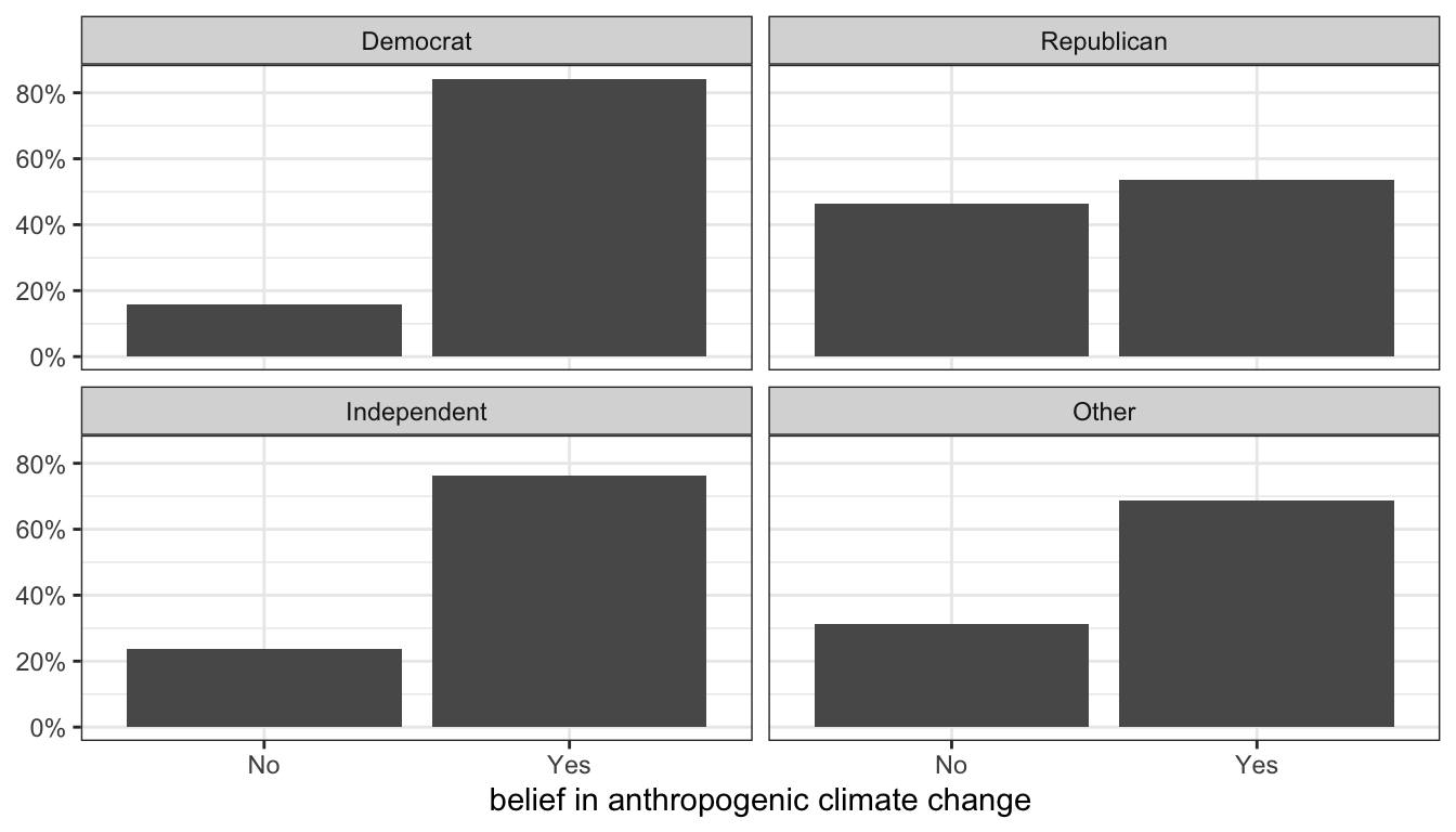
Figure 16: Distribution of belief in anthropogenic climate change by party affiliation, ANES 2016
Figure 16 is a comparative barplot. This is our first example of a graph that looks at a relationship. Each panel shows the distribution of climate change beliefs for respondents with that particular party affiliation. What we are interested in is whether the distribution looks different across each panel. In this case, because there were only two categories of the response variable, we only really need to look at the heights of the bar for one category to see the variation across party affiliation, which is substantial.
Lets try an example with more than two categories. For this example, I want to know whether there was a difference in passenger class by gender on the Titanic. I start with a comparative barplot:
ggplot(titanic, aes(x=pclass, y=..prop.., group=1))+
  geom_bar()+
  facet_wrap(~sex)+
  scale_y_continuous(labels = scales::percent)+
  labs(x="passenger class", y=NULL)+
  theme_bw()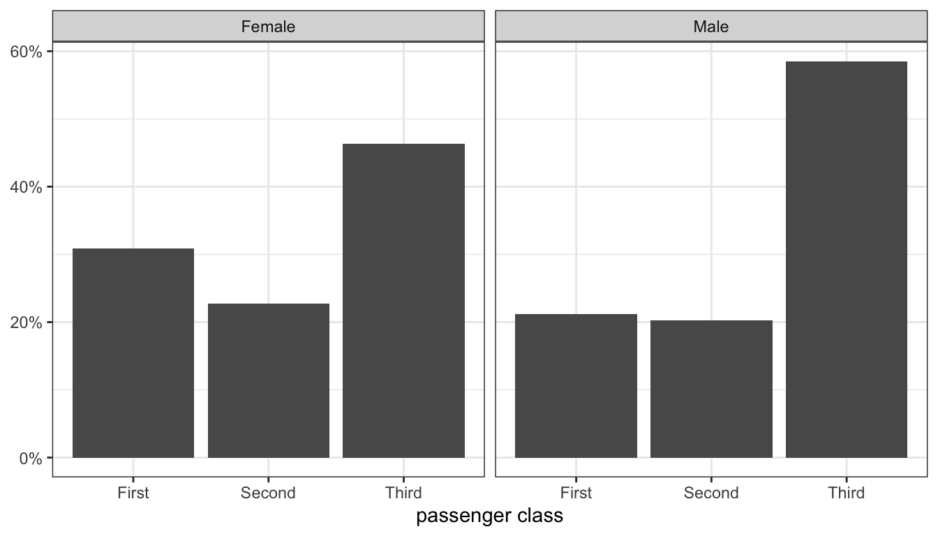
Figure 17: Distribution of passenger class by gender
I can also calculate the conditional distributions by hand using prop.table:
##
##          First Second Third
##   Female  30.9   22.7  46.4
##   Male    21.2   20.3  58.5
As these numbers and Figure 17 both show, the distribution of men and women by passenger class is very different. Women were less likely to be in third class and more likely to be in first class than men, while about the same percent of men and women were in second class.
Odds ratio (advanced)
We can also use the odds ratio to measure the association between two categorical variables. The odds ratio is not a term that is common in everyday speech but it is a critical concept in all kinds of scientific research.
Lets take the different distributions of climate change belief for Democrats and Republicans. About 84% of Democrats were believers, but only 54% of Republicans were believers. How can we talk about how different these two numbers are from one another? We could subtract one from the other or we could take the ratio by dividing one by the other. However, both of these approaches have a major problem. Because the percents (and proportions) have minimum and maximum values of 0 and 100, as you approach those boundaries the differences necessarily have to shrink because one group is hitting its upper or lower limit. This makes it difficult to compare percentage or proportional differences across different groups because the overall average proportion across groups will affect the differences in proportion.
Odds ratios are a way to get around this problem. To understand odds ratios, you first have to understand what odds are. All probabilities (or proportions) can be converted to a corresponding odds. If you have a \(p\) probability of success on a task, then your odds \(O\) of success are given by:
\[O=\frac{p}{1-p}\]
The odds are basically the ratio of the probability of success to the probability of failure. This tells you how many successes you expect to get for every one failure. Lets say a baseball player gets a hit 25% of the time that the player comes up to bat (an average of 250). The odds are then given by:
\[O=\frac{0.25}{1-0.25}=\frac{0.25}{0.75}=0.33333\]
The hitter will get on average 0.33 hits for every one out. Alternatively, you could say that the hitter will get one hit for every three outs.
Re-calculating probabilities in this way is useful because unlike the probability, the odds has no upper limit. As the probability of success approaches one, the odds will just get larger and larger.
We can use this same logic to construct the odds that a Democratic and Republican respondent, respectively, will be climate change believers. For the Democrat, the probability is 0.843, so the odds are:
\[O=\frac{0.843}{1-0.843}=\frac{0.843}{0.157}=5.369\]
Among Democrats, there are 5.369 believers for every one denier. Among Republicans, the probability is 0.541, so the odds are:
\[O=\frac{0.535}{1-0.535}=\frac{0.535}{0.465}=1.151\]
Among Republicans, there are 1.151 believers for every one denier. This number is close to “even” odds of 1, which happen when the probability is 50%.
The final step here is to compare those two odds. We do this by taking their ratio, which means we divide one number by the other:
\[\frac{5.369}{1.151}=4.67\]
This is our odds ratio. How do we interpret it? This odds ratio tells us how much more or less likely climate change belief is among Democrats relative to Republicans. In this case, I would say that “the odds of belief in anthropogenic climate change are 4.665 times higher among Democrats than Republicans.” Note the “times” here. This 4.665 is a multiplicative factor because we are taking a ratio of the two numbers.
You can calculate odds ratios from conditional distributions just as I have done above, but there is also a short cut technique called the cross-product. Lets look at the two-way table of party affiliation but this time just for Democrats and Republicans. For reasons I will explain below, I am going to reverse the ordering of the columns so that believers come first.
| Believer | Denier | |
|---|---|---|
| Democrat | 1235 | 230 |
| Republican | 664 | 577 |
The two numbers in blue are called the diagonal and the two numbers in red are the reverse diagonal. The cross-product is calculated by multiplying the two numbers in the diagonal by each other and multiplying the two numbers in the reverse diagonal together and then dividing the former product by the latter:
\[\frac{1235*577}{664*230}=4.67\]
I get the exact same odds ratio as above without having to calculate the proportions and odds themselves. This is a useful shortcut for calculating odds ratios.
The odds ratio that you calculate is always the odds of the first row being in the first column relative to those odds for the second row. Its easy to show how this would be different if I had kept the original ordering of believers and deniers:
| Denier | Believer | |
|---|---|---|
| Democrat | 230 | 1235 |
| Republican | 577 | 664 |
\[\frac{230*664}{577*1235}=0.21\]
I get a very different odds ratio, but that is because I am calculating something different. I am now calculating the odds ratio of being a denier rather than a believer. So I would say that the “the odds of denial of anthropogenic climate change among Democrats are only 22% of the odds for Republicans.” In other words, the odds of being a denier are much lower among Democrats.
However, the information here is the same because the 0.21 here is exactly equal to 1/4.67. In other words, the odds ratio of denial is just the inverted mirror image of the odds ratio of belief. Its just important that you remember that when you calculate the cross-product, you are always calculating the odds ratio of being in the category of the first column, whatever category that may be.