Hypothesis Tests
In social scientific practice, hypothesis testing is far more common than confidence intervals as a technique of statistical inference. Both techniques are fundamentally derived from the sampling distribution and produce similar results, but the methodology and interpretation of results is very different.
In hypothesis testing, we play a game of make believe. Remember that the fundamental issue we are trying to work around is that we don’t know the value of the true population parameter and thus we don’t know where the center is for the sampling distribution of the sample statistic. In hypothesis testing, we work around this issue by boldly asserting what we think the true population parameter. We then test whether the data that we got are reasonably consistent with that assertion.
Example: Coke winners
Lets take a fairly straightforward example. Coca-Cola used to run promotions where a certain percentage of bottle caps were claimed to win you another free coke. In one such promotion, when I was in graduate school, Coca-Cola ran a promotion where they claimed that 1 in 12 bottles were winners. If this is true, then 8.3% (1/12=0.083) of all the coke bottles in every grocery store and mini mart should be winners.
Being a grad student who needed to stay up late writing a dissertation fueled by caffeine and “sugar,” I use to drink quite a few Cokes. After only receiving a few winners after numerous attempts, I began to get suspicious of the claim. I started collecting bottle caps to see if I could statistically find evidence of fraudulent behavior.
For the sake of this exercise, lets say I collected 100 coke bottle caps (I never got this high in practice, but its a nice round number) and that I only got five winners. My winning percentage is 5% which is lower than Coke’s claim of 8.3%.
The critical question is whether it is likely or unlikely that I would get a winning percentage this different from the claim in a sample of 100 bottle caps. That is what a hypothesis test is all about. We are asking whether the data that we got are likely under some assumption about the true parameter. If they are unlikely, then we reject that assumption. if they are not unlikely, then we do not reject the assumption.
We call that assumption the null hypothesis, \(H_0\). The null hypothesis is a statement about what we think the true value of the parameter is. The null hypothesis is our “working assumption” until we can be proven to be wrong. In this case, the parameter of interest is the true proportion of winners among the population of all Coke bottles in the US. Coke claims that this proportion is 0.083, so this is my null hypothesis. In mathematical terms, we write:
\[H_0: \rho=0.083\]
I use the Greek letter \(\rho\) as a symbol for the population proportion. I will use \(\hat{p}\) to represent the sample proportion in my sample, which is 0.05.
Some standard statistical textbooks will also claim that there is an “alternative hypothesis.” That alternative hypothesis is specified as “anything but the null hypothesis.” In my opinion, this is incorrect because vague statements about “anything else” do not constitute an actual hypothesis about the data. We are testing only whether the data are consistent with the null hypothesis. No other hypothesis is relevant.
We got a sample proportion of 0.05 on a sample of 100. Assuming the null hypothesis is true, what would the sampling distribution look like from which I pulled my 0.05? Note the part in bold above. We are now playing our game of make believe.
We know that on a sample of 100, the sample proportion should be normally distributed. It should also be centered on the true population proportion. Because we are assuming the null hypothesis is true, it should be centered on the value of 0.083. The standard error of this sampling distribution is given by:
\[\sqrt{\frac{0.083*(1-0.083)}{100}}=0.028\]
Therefore, we should have a sampling distribution that looks like:
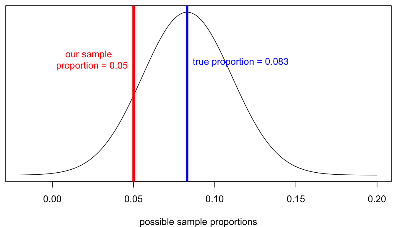
Figure 40: A game of make believe, or the sampling distribution for sample proportion of winning Coca-Cola bottle caps assuming the null hypothesis is true
The blue line shows the true population proportion assumed by the null hypothesis. The red line shows my actual sample proportion. The key question of hypothesis testing is whether the observed data (or more extreme data) are reasonably likely under the assumption of the null hypothesis. Practically speaking, I want to know how far my sample proportion is from the true proportion and whether this distance is far enough to consider it unlikely.
To calculate how far away I am on some standard scale, I divide the distance by the standard error of the sampling distribution to calculate how many standard errors my sample proportion is below the population parameter (assuming the null hypothesis is true).
\[\frac{0.05-0.083}{0.028}=\frac{-0.033}{0.028}=-1.18\]
My sample proportion is 1.18 standard errors below the center of the sampling distribution. Is this an unlikely distance? To figure this out, we need to calculate the area in the lower tail of the sampling distribution past my red line. This number will tell us the proportion of all sample proportions that would be 0.05 or lower, assuming the null hypothesis is true. This standardized measure of how far is sometimes called the test statistic for a given hypothesis test.
Calculating this area is not a trivial exercise, but R provides a straightforward command called pt which is somewhat similar to the qt command above. We just need to feed in how many standard errors our estimate is away from the center (-1.18) and the degrees of freedom. These degrees of freedom are identical to the ones used in confidence intervals (in this case, \(n-1\), so 99).
## [1] 0.1204139There is one catch with this command. It always gives you the area in the lower tail, so if your sample statistic is above the center, you should still put in a negative value in the first command. We will see an example of this below.
Our output indicates that 12% of all samples would produce a sample proportion of 0.05 or less when the true population proportion is 0.083. Graphically it looks like this:
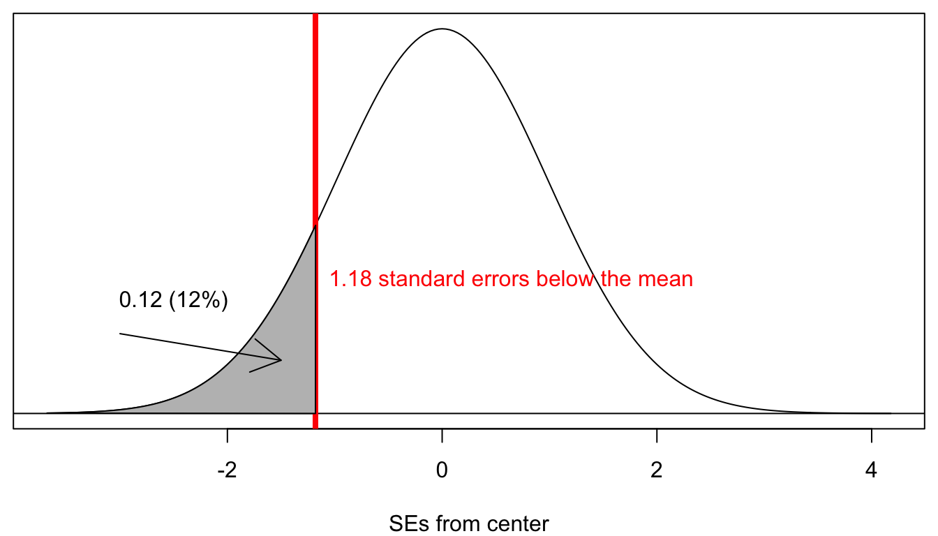
Figure 41: The proportion of all possible sample proportions that are lower than our sample proportion, assuming the null hypothesis is true
The grey area is the area in the lower tail. It would seem that we are almost ready to conclude our hypothesis test. However, there is a catch and its a tricky one. Remember that I was interested in the probability of getting a sample proportion this far or farther from the true population proportion. This is not the same as getting a sample proportion this low or lower. I need to consider the possibility that I would have been equally suspicious if I had got a sample proportion much higher than 8.3%. In mathematically terms, that means I need to take the area in the upper tail as well, where I am .033 above the true population proportion. This is called a two-tailed test. Luckily, because the normal distribution is symmetric, this area will be identical to the area in the lower tail and so I can just double this percent.
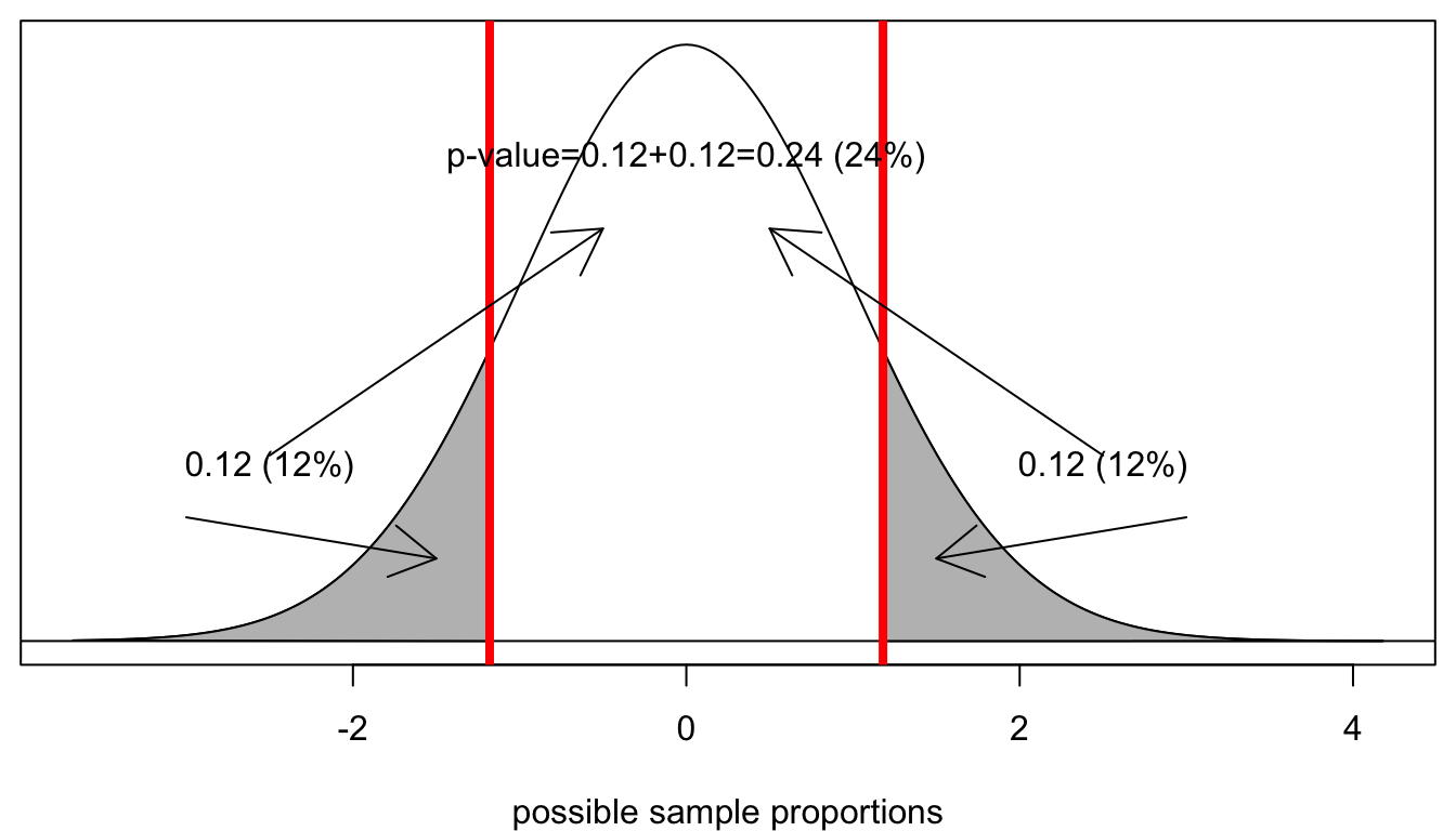
Figure 42: We have to also consider the possibility of getting a sample proportion as far from the population proportion but in the other direction
Assuming the null hypothesis is true, there is a 24% chance of getting a sample proportion as far from the true population mean or farther, just by random chance. We call this probability the p-value. The p-value is the ultimate goal of the hypothesis test. All hypothesis tests produce a p-value and it is the p-value that we will use to make a decision about our test.
What should that decision be? We have only two choices. If the p-value is low enough, then it is unlikely that we would have gotten this data or data more extreme, assuming the null hypothesis is true. Therefore, we reject the null hypothesis. If the p-value is not low enough, then it is reasonable that we would have gotten this data or data more extreme, assuming the null hypothesis is true. Therefore, we fail to reject the null hypothesis. Note that we NEVER accept or prove the null hypothesis. It is already our working assumption, so the best we can do for it is to fail to reject it and thus continue to use it as our working assumption.
How low does the p-value need to be in order to reject it? There is no right answer here, because this is a subjective question. However, there is a generally agreed upon practice in the social sciences that we reject the null hypothesis when the p-value is at or below 0.05 (5%). Note that while there is general consensus around this number, it is an arbitrary cutpoint. The practical difference between a p-value of 0.049 and 0.051 is negligible, but under this arbitrary standard, we would make different decisions in each case. I would rather that you just learn to think about what the p-value represents and reach your own decision.
No reasonable scientist, however, would reject the null hypothesis with a p-value of 24% as we have in our Coke case. Nearly 1 in 4 samples of size 100 would produce a sample proportion this different from the assumed true proportion of 8.3% just by random chance. I therefore do not have sufficient evidence to reject the null hypothesis that Coke is telling the truth. Note that I have not proved that Coke is telling the truth. I have only failed to produce evidence that they are lying.
The general procedure of hypothesis testing
The general procedure of hypothesis testing is as follows:
- State a null hypothesis. This null hypothesis is a claim about the true value of an unknown parameter.
- Calculate a test statistic that tells you how far your sample statistic is from the center of the sampling distribution, assuming the null hypothesis is true. For our purposes, this test statistic will always be the number of standard errors above or below the true population parameter, assuming the null hypothesis is true.
- Calculate the p-value for the test statistic. The p-value is the probability of getting a sample statistic this far or farther (in absolute value) from the true population parameter, assuming the null hypothesis is true.
- If the p-value is below some threshold (typically 0.05), reject the null hypothesis. Otherwise, fail to reject the null hypothesis.
Interpreting p-values correctly
P-values are widely misunderstood in practice. Studies have been done of practicing researchers across different disciplines where these researchers were asked to interpret a p-value from a multiple choice question and the majority get it wrong. Therefore, don’t feel bad if you are having trouble understanding a p-value. You are in good company! Nonetheless, proper interpretation of a p-value is critically important for our understanding of what a hypothesis test does.
The reason many people get the interpretation of p-values wrong is that they want the p-value to express the probability of a hypothesis being correct or incorrect. People routinely misinterpret the p-value as a statement about the probability of the null hypothesis being correct. The p-value is NOT a statement about the probability of a hypothesis being correct or incorrect. For the same reason that we cannot call a confidence interval a probability statement, the classical approach dictates that we cannot characterize our subjective uncertainty about whether hypotheses are true or not by a probability statement. The hypothesis is either correct or it is not. There is no probability.
Correctly interpreted, the p-value is a probability statement about the data, not about the hypothesis. Specifically, we are asking what the probability is of observing data this extreme or more extreme, assuming the null hypothesis is true. We are not making a probability statement about hypotheses. Rather we are assuming a hypothesis and then asking about the probability of the data. This difference may seem subtle, but it is in fact quite substantial in interpretation.
The reason why everyone (including you and me) struggles with this is that our brains want it to be the other way around. Ultimately by rejecting or failing to reject we are making statements about whether we believe the hypothesis or not, but we are not doing that directly by a probability statement about the hypothesis but rather a probability statement about the likelihood of the data given the hypothesis.
Hypothesis tests of relationships
The hypothesis tests that we care the most about in the sciences are hypothesis tests about relationships between variables. We want to know whether the association we are observing in the sample is true in the population. In all of these cases, our null hypothesis is that there is no association, and we want to know whether the association we observe in the sample is strong enough to reject this null hypothesis of no association. We can do hypothesis tests of this nature for both mean differences and regression slopes.
Example: mean differences
Lets look at differences in mean income (measured in $1000) by religion in the politics dataset.
##    Mainline Protestant Evangelical Protestant               Catholic
##               81.83439               58.32606               77.53498
##                 Jewish          Non-religious                  Other
##              120.92958               88.62963               60.75311
I want to look at the difference between Evangelical Protestants and “Other Religions.” The mean difference here is:
\[58.32606-60.75311=-2.42705\]
Evangelical Protestants make $2,427 less than members of other religions, in my sample.
Let me set up a hypothesis test where the null hypothesis is that Roman Catholics and members of other religions have the same income, or in other words, the mean difference in income is zero:
\[H_0: \mu_c-\mu_o=0\]
Where \(\mu_c\) is the population mean income of evangelical Protestants and \(\mu_o\) is the population mean income of members of other religions. In order to figure out how far my sample mean difference of -2.427 is from 0, I need to find the standard error of the mean difference. The formula for this number is:
\[\sqrt{\frac{s_c^2}{n_c}+\frac{s_o^2}{n_o}}\]
I can calculate this in R:
##    Mainline Protestant Evangelical Protestant               Catholic
##               62.90763               51.23396               66.59281
##                 Jewish          Non-religious                  Other
## 89.84166 71.46392 56.37886##
## Mainline Protestant Evangelical Protestant Catholic
## 785 917 1015
## Jewish Non-religious Other
## 71 567 883## [1] -0.9547436The t-statistic of -0.95 here is not very large. I am only 0.44 standard errors below 0 on the sampling distribution, assuming the null hypothesis is true. Lets go ahead and calculate the p-value for this t-statistic. Remember that I need to put in the negative version of this number to the pt command. I also need to use the smaller of the two sample sizes for my degrees of freedom:
## [1] 0.3423725In a sample of this size, there is an 34% chance of observing a mean income difference of $2,427 or more between evangelical Protestants and members of other religions, just by sampling error, assuming that there is no difference in income in the population. Therefore, I fail to reject the null hypothesis that evangelical Protestants and members of other religions make the same income.
Example of proportion differences
Lets look at the difference in smoking behavior between white and black students in the Add Health data. Our null hypothesis is:
\[H_0: \rho_w-\rho_c=0\] In simple terms, our null hypothesis is that the same proportion of white and black adolescents smoke frequently. Lets look at the actual numbers from our sample:
##
##                   White  Black/African American     Latino
##   Non-smoker 0.79560106              0.94847162 0.89000000
##   Smoker     0.20439894              0.05152838 0.11000000
##
##               Asian/Pacific Islander      Other
##   Non-smoker              0.90123457 0.92592593
##   Smoker                  0.09876543 0.07407407
##
##               American Indian/Native American
##   Non-smoker                       0.80769231
## Smoker 0.19230769## [1] 0.1528706About 20.4% of white students smoked frequently, compared to only 5.2% of black students. The difference in proportion is a large 15.3% in the sample. This would seem to contradict our null hypothesis. However, we need to confirm that a difference this large in a sample of our size is unlikely to happen by random chance. To do that we need to calculate the standard error, just as we learned to do it for proportion differences in the confidence interval section:
##
##                            White           Black/African American
##                             2637                             1145
##                           Latino           Asian/Pacific Islander
##                              400                              162
##                            Other  American Indian/Native American
## 27 26## [1] 0.01021531Now many standard errors is our observed difference in proportion from zero?
## [1] 14.96485Wow, thats a lot. We can be pretty confident already without the final step of the p-value, but lets calculate it anyway. Remember ot always take the negative version of the t-statistic you calculated:
## [1] 2.247969e-46The p-value is astronomically small. In a sample of this size, the probability of observing a difference in the proportion frequent smokers between whites and blacks of 15.3% or larger if there is no difference in the population is less than 0.0000001%. Therefore, I reject the null hypothesis and conclude that white students are more likely to be frequent smokers than are black students.
Example of correlation coefficient
Lets look at the correlation between the parental income of a student and the number of friend nominations they receive. Our null hypothesis will be that there is no relationship between parental income and student popularity in the population of US adolescents. Lets look at the data in our sample:
## [1] 0.1247392In the sample we observe a moderately positive correlation between a student’s parental income and the number of friend nominations they receive. How confident are we that we wouldn’t observe such a large correlation coefficient in our sample by random chance if the null hypothesis is true?
First, we need to calculate the standard error:
## [1] 0.01496633How many standard errors are we away from the assumption of zero correlation?
## [1] 8.334658What is the probability of being that far away from zero for a sample of this size?
## [1] 1.027779e-16The probability is very small. In a sample of this size, the probability is less than 0.00000001% of observing a correlation coefficient between parental income and friend nominations received of an absolute magnitude of 0.125 or higher when the true correlation is zero in the population. Therefore, we reject the null hypothesis and conclude that there is a positive correlation between parental income and popularity among US adolescents.
Statistical Significance
When a researcher is able to reject the null hypothesis of “no association,” the result is said to be statistically significant. This is a somewhat unfortunate phrase that is sometimes loosely interpreted to indicate that the result is “important” in some vague scientific sense.
In practice, it is important to distinguish between substantive and statistical significance. In very large datasets, standard errors will be very small, and thus it is possible to observe associations that are very small in substantive size that are nonetheless statistically significant. On the flip side, in small datasets, standard errors will often be large, and thus it is possible to observe associations that are very large in substantive size but not statistically significant.
It is important to remember that “statistical significance” is a reference to statistical inference and not a direct measure of the actual magnitude of an association. I prefer the term “statistically distinguishable” to “statistically significant” because it more clearly indicates what is going on. In the previous example, we found that the income differences in our sample between Catholics and members of other religions are not statistically distinguishable from zero. We also found that the negative association in our sample between age and sexual frequency was statistically distinguishable from zero. Establishing whether an association is worthwhile in its substantive effect is a totally different exercise from establishing whether it is statistically distinguishable from zero.
It is also important to remember that a statistically insignificant finding is not evidence of no relationship because we never accept the null hypothesis. We have just failed to find sufficient evidence of a relationship. No evidence of an association is not evidence of no association.