Confidence Intervals
As Figure 38 shows, 95% of all the possible sample means will be within 1.96 standard errors of the true population mean \(\mu\).
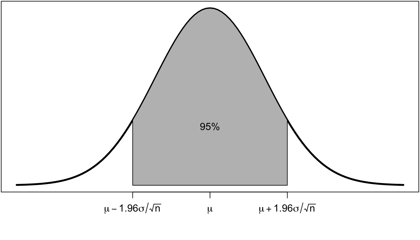
Figure 38: 95% of all sample means will be within 1.96 standard errors of the true population mean.
Lets say I were to construct the following interval for every possible sample:
\[\bar{x}\pm1.96(\sigma/\sqrt{n})\]
It follows from the statement above that for 95% of all samples, this interval would contain the true population mean, \(\mu\).
To see how this works graphically, imagine constructing this interval for twenty different samples from the same population. Figure 39 shows the mean and interval for each of these twenty samples, relative to the true population mean.
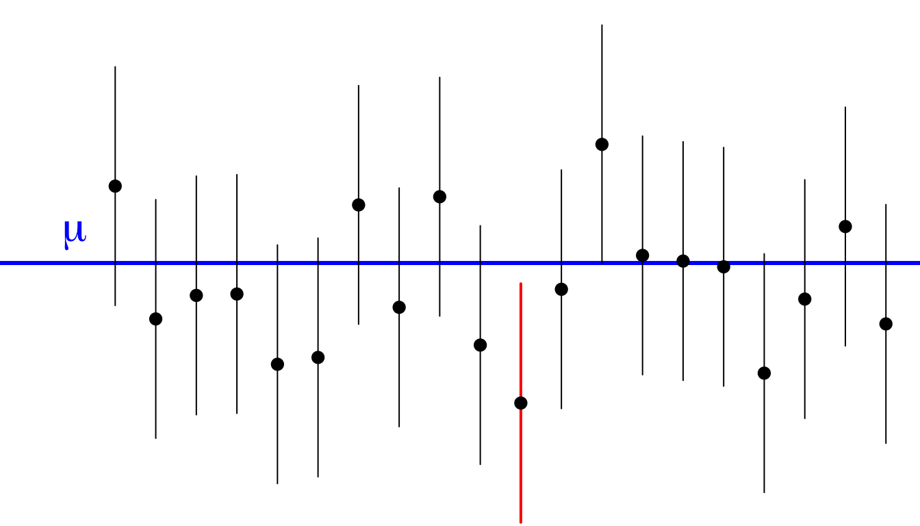
Figure 39: Intervals of sample mean plus and minus 1.96 standard errors for 20 different samples, with the true population mean shown by the blue line. Sample means shown by dots.
You can see that these sample means fluctuate around the true population mean due to random sampling error. The lines give the interval outlined above. In 19 out of the 20 cases, this interval contains the true population mean (as you can see by the fact that the interval crosses the blue line). The one sample where this is not true is shown in red. On average, 95% of samples will contain the true population mean in the interval, so 5% or 1 in 20 will not.
We refer to this interval as the 95% confidence interval. Of course, in practice, we only construct one interval on the sample that we have. We use this interval to give a range of values that we feel “confident” will contain the true population mean.
What do we mean by “confident?”
The term “confident” is a little ambiguous. Given my statements above, it might be tempting to interpret the 95% confidence interval to mean that there is a 95% probability that the true population mean is within the interval. This interpretation seems intuitive and straightforward, but that interpretation is incorrect according to the classic approach to inference. The problem here is subtle, but from the classical viewpoint, probability is an objective phenomenon that relates to the outcomes of future processes over the long run. From this viewpoint, we cannot express our subjective uncertainties about numbers in terms of probabilities.The population mean is a single static number. This leads us to a sort of yoda-like statement: The population mean is either in your interval or it is not. There is no probability.
This is why we use a more neutral term like “confidence.” If we want to be long-winded about it, we might say that we are 95% confident because “in 95% of all the possible samples I could have drawn, the true population mean would be in the interval. I don’t know if I have one of those 95% or the unlucky 5%, but nonetheless, there it is.”
If this all seems a bit confusing, you are perfectly normal. As I said, this is the classic view of probability. Intuitively, people often think of uncertainty in probabilistic terms (e.g. what are the odds your team will win the game?). Many contemporary statisticians would in fact agree that it is perfectly okay to express subjective uncertainty as a probability. But, I still need to let you know that from the classic approach, interpreting your confidence interval as a probability statement is a no-no.
Calculating the confidence interval for the sample mean
Okay, lets try calculating a confidence interval. Lets try this out for age in the politics dataset. The formula is:
\[\bar{x}\pm1.96(\sigma/\sqrt{n})\]
Oh wait, we can’t do it! We don’t know the value of the population standard deviation \(\sigma\). As I explained in the last section, we are going to have to do a little “fudging” here. Instead of \(\sigma\), we can use our sample standard deviation \(s\). However, doing so will have consequences. Here is our new formula:
\[\bar{x} \pm t*(s\sqrt{n})\]
As you can see, I have replaced the 1.96 with some number \(t\), referred to as the t-statistic. Basically to adjust for the greater uncertainty in using a sample statistic in my calculation of the standard error, I need to increase the number here slightly from 1.96. How much I increase it will depend on the degrees of freedom which are given by the sample size minus one (\(n-1\)). To figure out the correct t-statistic, I can use the qt command in R.
## [1] 1.960524The first command to qt is the confidence you want. This is a little bit tricky because for a 95% confidence interval, we actually want to input 0.975. This is because we are basically asking for only the upper tail of that normal distribution shown at the beginning of this section. This area contains only 2.5% of the area outside, with the other 2.5% being in the lower tail. The second number is the degrees of freedom which equals \(n-1\). In this case, we have such a large sample, that the t-statistic we need is very close to 1.96.
In smaller samples, using the t-statistic rather than 1.96 can make a bigger difference. Its not a proper sample, but lets take the case of the crime data. Here there are only 51 observations, so the t-statistic is:
## [1] 2.008559The difference from 1.96 is a little more noticeable.
Lets return to the politics data. We now have all the information we need to calculate the 95% confidence interval:
xbar <- mean(politics$age)
sdx <- sd(politics$age)
n <- nrow(politics)
se <- sdx/sqrt(n)
t <- qt(0.975,n-1)
xbar+t*se
## [1] 50.03165## [1] 48.97307We are 95% confident that the mean age among all US adults is between 48.97 and 50.03 years of age. As you can see, the large sample of nearly 6,000 respondents produces a very tight confidence interval.
Calculating the confidence interval for other sample statistics
As noted in the previous section, the sampling distribution of other sample statistics such as proportions, mean differences, and regression slopes is also normally distributed in large enough samples. This means that we can use the same approach to construct confidence intervals for other sample statistics. The general form of the confidence interval is:
\[\texttt{(sample statistic)} \pm t*\texttt{(standard error)}\]
In order to do this for any of the above sample statistics, we only need to know how to calculate that sample statistic’s standard error and the degrees of freedom used to look up the t-statistic for that sample statistic. Table 12 provides a useful cheat sheet of those formulas:
| Type | SE | df for \(t\) |
|---|---|---|
| Mean | \(s/\sqrt{n}\) | \(n-1\) |
| Proportion | \(\sqrt\frac{\hat{p}*(1-\hat{p})}{n}\) | \(n-1\) |
| Mean Difference | \(\sqrt{\frac{s_1^2}{n_1}+\frac{s_2^2}{n_2}}\) | min(\(n_1-1\),\(n_2-1\)) |
| Proportion Difference | \(\sqrt{\frac{\hat{p}_1*(1-\hat{p}_1)}{n_1}+\frac{\hat{p}_2*(1-\hat{p}_2)}{n_2}}\) | min(\(n_1-1\),\(n_2-1\)) |
| Correlation Coefficient | \(\sqrt{\frac{1-r^2}{n-2}}\) | \(n-2\) |
I know some of that math might look intimidating but I will go through an example of each case below to show you how it works for each case.
Example with proportions
As an example, lets use the proportion of respondents who do not believe in anthropogenic climate change. In our politics sample, we get:
##
##   No  Yes
## 1180 3058## [1] 4238## [1] 0.2784332About 27.8% of the respondents in our sample are climate change deniers. What can we conclude about the proportion in the US population? First, lets figure out the t-statistic. We use the same \(n-1\) for degrees of freedom:
## [1] 1.960524Our sample is large enough that we are basically using 1.96. Now we need to calculate the standard error. The formula from above is:
\[\sqrt{\frac{\hat{p}*(1-\hat{p})}{n}}\]
The term \(hat{p}\) is the standard way to represent the sample proportion, which in this case is 0.279. So, our formula is:
\[\sqrt{\frac{0.278*(1-0.278)}{4238}}\]
We can calculate this in R:
## [1] 0.006885228We now have all the pieces to construct the confidence interval:
## [1] 0.2919319## [1] 0.2649346We are 95% confident that the true percentage of climate change deniers in the the US population is between 26.5% and 29.2%.
Example with mean differences
using our Add health data, what is the mean difference in popularity (number of friend nominations) between frequent smokers and those who do not smoke frequently?
## Non-smoker     Smoker
## 4.506699 4.796992## [1] 0.290293In our sample data, frequent smokers had 0.290 more friends on average than those who did not smoke frequently. What is the confidence interval for that value in the population? We start by calculating the t-statistic for this confidence interval. We use the size of the smaller group minus one for the degrees of freedom.
##
## Non-smoker     Smoker
## 3732 665## [1] 1.963543The value is pretty close to 1.96 but a little bigger. Now we need to calculate the standard error. The formula is:
\[\sqrt{\frac{s_1^2}{n_1}+\frac{s_2^2}{n_2}}\]
We already have \(n_1\) and \(n_2\), so we just need to get the standard deviation of friend nominations for the two groups to get \(s_1\) and \(s_2\). We can do this with another tapply command, but changing from mean to sd in the third argument.
## Non-smoker     Smoker
## 3.652224 3.901188## [1] 0.1626661Now we have all the pieces to put together the confidence interval:
## [1] -0.02910896## [1] 0.609695We are 95% confident that in the population of US adolescents, those who smoke frequently have between 0.03 fewer to 0.61 more friend nominations, on average, than those who do not smoke frequently. Note that because our confidence interval contains both negative and positive value, we cannot be confident about whether smoking is truly associated with having more or less friends. The direction of the relationship between the two variables is uncertain.
Example with proportion differences
Lets continue to use the Add Health data. Do we observe a gender difference in smoking behavior in our sample?
##
##                 Female      Male
##   Non-smoker 0.8534894 0.8435407
## Smoker 0.1465106 0.1564593## [1] 0.0099487In our sample, about 14.7% of girls were frequent smokers and about 15.6% of boys were frequent smokers. The percentage of boys who smoke is about 1% higher than the percentage of girls. Do we think this moderate difference in the sample is true in the population?
Lets start again by calculating the appropriate t-statistic for our confidence interval. We use the same procedure as for mean differences above, choosing the size of the smaller group for the degrees of freedom. However, its important to note that our groups are now boys and girls, not smokers and non-smokers.
##
##  Female    Male
## 2307 2090## [1] 1.9611Now we can calculate the standard error. The formula is:
\[\sqrt{\frac{\hat{p}_1*(1-\hat{p}_1)}{n_1}+\frac{\hat{p}_2*(1-\hat{p}_2)}{n_2}}\]
That looks like a lot, but we just have to focus on plugging in the right values in R:
## [1] 0.01083286Now we have all the parts to calculate the confidence interval:
## [1] -0.01129562## [1] 0.03119302We are 95% confident that in the population of US adolescents, between 1.1% fewer to 3.1% more boys smoke frequently than girls. As above, because our confidence interval includes both negative and positive values, we are not very confident at all about whether boys or girls smoke more frequently.
Example with correlation coefficient
Lets stick with the Add Health data. What is the correlation between GPA and the number of friend nominations that a student receives?
## [1] 0.1680881In our sample, there is a moderately positive correlation between a student’s GPA and the number of friend nominations that a student receives. What is our confidence interval for the population?
For the t-statistic, we use \(n-2\) for the degrees of freedom:
For the standard error, the formula is:
\[\sqrt{\frac{1-r^2}{n-2}}\] This is straightforward to calculate in R:
## [1] 0.01486952Now we have all the parts we need to calculate the confidence interval:
## [1] 0.1389363## [1] 0.1972398We are 95% confident that the true correlation coefficient between GPA and friend nominations in the population of US adolescents is between 0.139 and 0.197. While there is some difference in the strength of that relationship, we are pretty confident that the correlation is moderately positive.