The Linear Model, Revisited
Reformulating the linear model
Up until now, we have used the following equation to describe the linear model mathematically:
\[\hat{y}_i=\beta_0+\beta_1x_{i1}+\beta_2x_{i2}+\ldots+\beta_px_{ip}\] In this formulation, \(\hat{y}_i\) is the predicted value of the dependent variable for the \(i\)th observation and \(x_{i1}\), \(x_{i2}\). through \(x_{ip}\) are the values of \(p\) independent variables that predict \(\hat{y}_i\) by a linear function. \(\beta_0\) is the y-intercept which is the predicted value of dependent variable when all the independent variables are zero. \(\beta_1\) through \(\beta_p\) are the slopes giving the predicted change in the dependent variable for a one unit increase in a given independent variable holding all of the other variables constant.
This formulation is useful, but we can now expand and re-formulate it in a way that will help us understand some of the more advanced topics we will discuss in this and later chapters. The formula is above is only the “structural” part of the full linear model. The full linear model is given by:
\[y_i=\beta_0+\beta_1x_{i1}+\beta_2x_{i2}+\ldots+\beta_px_{ip}+\epsilon_i\]
I have changed two things in this new formula. On the left-hand side, we have the actual value of the dependent variable for the \(i\)th observation. In order to make things balance on the right-hand side of the equation, I have added \(\epsilon_i\) which is simply the residual or error term for the \(i\)th observation. We now have a full model that predicts the actual values of \(y\) from the actual values of \(x\).
If we compare this to the first formula, it should become clear that every term except the residual term can be substituted for by \(\hat{y}_i\). So, we can restate our linear model using two separate formulas as follows:
\[\hat{y}_i=\beta_0+\beta_1x_{i1}+\beta_2x_{i2}+\ldots+\beta_px_{ip}\]
\[y_i=\hat{y}_i+\epsilon_i\]
By dividing up the formula into two separate components, we can begin to think of our linear model as containing a structural component and a random (or stochastic) component. The structural component is the linear equation predicting \(\hat{y}_i\). This is the formal relationship we are trying to fit between the dependent and independent variables. The stochastic component on the other hand is given by the \(\epsilon_i\) term in the second formula. In order to get back to the actual values of the dependent variable, we have to add in the residual component that is not accounted for by the linear model.
From this perspective, we can rethink our entire linear model as a partition of the total variation in the dependent variable into the structural component that can be accounted for by our linear model and the residual component that is unaccounted for by the model. This is exactly as we envisioned things when we learned to calculate \(R^2\) in previous chapters.
Marginal effects
The marginal effect of \(x\) on \(y\) gives the expected change in \(y\) for a one unit increase in \(x\) at a given value of \(x\). If that sounds familiar, its because this is very similar to the interpretation we give of the slope in a linear model. In a basic linear model with no interaction terms, the marginal effect of a given independent variable is in fact given by the slope.
The difference in interpretation is the little part about “at a given value of x.” In a basic linear model this addendum is irrelevant because the expected increase in \(y\) for a one unit increase in \(x\) is the same regardless of the current value of \(x\) – thats what it means for an effect to be linear. However, when we start delving into more complex model structures, such as interaction terms and some of the models we will discuss in this module, things get more complicated. The marginal effect can help us make sense of complicated models.
The marginal effect is calculated using calculus. I won’t delve too deeply into the details here, but the marginal effect is equal to the partial derivative of y with respect to x. This partial derivative gives us what is called the tangent line of a curve at any point of \(x\) which measures the instantenous rate of change in some mathematical function.
Lets take the case of a simple linear model with two predictor variables:
\[y_i=\beta_0+\beta_1x_{i1}+\beta_2x_{i2}+\epsilon_i\]
We can calculate the marginal effect of \(x_1\) and \(x_2\) by taking their partial derivatives. If you don’t know how to do that, its fine. But if you do know a little calculus, this is a simple calculation:
\[\frac{\partial y}{\partial x_1}=\beta_1\] \[\frac{\partial y}{\partial x_2}=\beta_2\]
As stated above, the marginal effects are just given by the slope for each variable, respectively.
Marginal effects really become useful when we have more complex models. Lets now try a model similar to the one above but with an interaction term:
\[y_i=\beta_0+\beta_1x_{i1}+\beta_2x_{i2}+\beta_3x_{i1}x_{i2}+\epsilon_i\]
The partial derivatives of this model turn out to be:
\[\frac{\partial y}{\partial x_1}=\beta_1+\beta_3x_{i2}\] \[\frac{\partial y}{\partial x_2}=\beta_2+\beta_3x_{i1}\]
The marginal effect of each independent variable on \(y\) now depends on the value of the other independent variable. Thats how interaction terms work, but now we can see that effect much more clearly in a mathematical sense. The slope of each independent variable is itself determined by a linear function rather than being a single constant value.
Marginal effect interaction example
Lets try this with a concrete example. For this case, I will look at the effect on wages of the interaction between number of children in the household and gender:
##         (Intercept)              nchild        genderFemale nchild:genderFemale
##              24.720               1.779              -2.839              -1.335
So, my full model is given by:
\[\hat{\text{wages}}_i=24.720+1.779(\text{nchildren}_i)-2.839(\text{female}_i)-1.335(\text{nchildren}_i)(\text{female}_i)\]
Following the formulas above, the marginal effect of number of children is given by:
\[1.779-1.335(\text{female}_i)\]
Note that this only takes two values because female is an indicator variable. When we have a man, the \(\text{female}\) variable will be zero and therefore the effect of an additional child will be 1.779. When we have a woman, \(\text{female}\) variable will be one, and the effect of an additional child will be \(1.779-1.335=0.444\).
The marginal effect for the gender gap will be given by:
\[-2.839-1.335(\text{nchildren}_i)\]
So the gender gap starts at 2.839 with no children in the household and grows by 1.335 for each additional child.
We can also plot up a marginal effects graph that shows us how the gender gap changes by number of children in the household.
nchild <- 0:6
gender_gap <- -2.839-1.335*nchild
df <- data.frame(nchild, gender_gap)
ggplot(df, aes(x=nchild, y=gender_gap))+
  geom_line(linetype=2, color="grey")+
  geom_point()+
  labs(x="number of children in household",
       y="predicted gender gap in hourly wages")+
  scale_y_continuous(labels = scales::dollar)+
  theme_bw()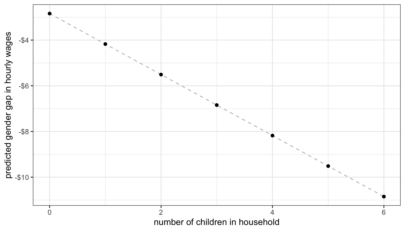
Figure 56: Marginal effect of number of children on the gender gap in wages
Linear model assumptions
Two important assumptions underlie the linear model. The first assumption is the assumption of linearity. In short, we assume that the the relationship between the dependent and independent variables is best described by a linear function. In prior chapters, we have seen examples where this assumption of linearity was clearly violated. When we choose the wrong model for the given relationship, we have made a specification error. Fitting a linear model to a non-linear relationship is one of the most common forms of specification error. However, this assumption is not as deadly as it sounds. Provided that we correctly diagnose the problem, there are a variety of tools that we can use to fit a non-linear relationship within the linear model framework. We will cover this techniques in the next section.
The second assumption of linear models is that the residual or error terms \(\epsilon_i\) are independent of one another and identically distributed. This is often called the i.i.d. assumption, for short. This assumption is a little more subtle. In order to understand, we need to return to this equation from earlier:
\[y_i=\hat{y}_i+\epsilon_i\]
One way to think about what is going on here is that in order to get an actual value of \(y_i\) you feed in all of the independent variables into your linear model equation to get \(\hat{y}_i\) and then you reach into some distribution of numbers (or a bag of numbers if you need something more concrete to visualize) to pull out a random value of \(\epsilon_i\) which you add to the end of your predicted value to get the actual value. When we think about the equation this way, we are thinking about it as a data generating process in which we get \(y_i\) values from completing the equation on the right.
The i.i.d. assumption comes into play when we reach into that distribution (or bag) to draw out our random values. Independence assumes that what we drew previously won’t affect what we draw in the future. The most common violation of this assumption is in time series data in which peaks and valleys in the time series tend to come clustered in time, so that when you have a high (or low) error in one year, you are likely to have a similar error in the next year. Identically distributed means that you are drawn from the same distribution (or bag) each time you make a draw. One of the most common violation of this assumption is when error terms tend to get larger in absolute size as the predicted value grows in size.
In later sections of this chapter, we will cover the i.i.d. assumption in more detail including the consequences of violating it, diagnostics for detecting it, and some corrections for when it does occur.
Estimating a linear model
Up until now, we have not discussed how R actually calculates all of the slopes and intercept for a linear model with multiple independent variables. We only know the equations for a linear model with one independent variable.
Even though we don’t know the math yet behind how linear model parameters are estimated, we do know the rationale for why they are selected. We choose the parameters that minimized the sum of squared residuals given by:
\[\sum_{i=1}^n (y_i-\hat{y}_i)^2\] In this section, we will learn the formal math that underlies how this estimation occurs, but first a warning: there is a lot of math ahead. In normal everyday practice, you don’t have to do any of this math, because R will do it for you. However, it is useful to know how linear model estimating works “under the hood” and it will help with some of the techniques we will learn later in the book.
Matrix algebra crash course
In order to learn how to estimate linear model parameters, we will need to learn a little bit of matrix algebra. In matrix algebra we can collect numbers into vectors which are single dimension arrays of numbers and matrices which are two-dimensional arrays of numbers. We can use matrix algebra to represent our linear regression model equation using one-dimensional vectors and two-dimensional matrices. We can imagine \(y\) below as a vector of dimension 3x1 and \(\mathbf{X}\) as a matrix of dimension 3x3.
\[ \mathbf{y}=\begin{pmatrix} 4\\ 5\\ 3\\ \end{pmatrix} \mathbf{X}= \begin{pmatrix} 1 & 7 & 4\\ 1 & 3 & 2\\ 1 & 1 & 6\\ \end{pmatrix} \]
We can multiply vectors and matrices together by taking each element in the row of a matrix by the corresponding element in the vector and summing them up:
\[\begin{pmatrix} 1 & 7 & 4\\ 1 & 3 & 2\\ 1 & 1 & 6\\ \end{pmatrix} \begin{pmatrix} 4\\ 5\\ 3\\ \end{pmatrix}= \begin{pmatrix} 1*4+7*5+3*4\\ 1*4+3*5+2*3\\ 1*4+1*5+6*3\\ \end{pmatrix}= \begin{pmatrix} 51\\ 25\\ 27\\ \end{pmatrix}\]
You can also transpose a vector or matrix by flipping its rows and columns. My transposed version of \(\mathbf{X}\) is \(\mathbf{X}'\) which is:
\[\mathbf{X}= \begin{pmatrix} 1 & 1 & 1\\ 7 & 3 & 1\\ 4 & 2 & 6\\ \end{pmatrix}\]
You can also multiple matrices by each other using the same pattern as for multiplying vectors and matrices but now you start a new column each time you move down a row of the first matrix. So to “square” my matrix:
\[ \begin{eqnarray*} \mathbf{X}'\mathbf{X}&=& \begin{pmatrix} 1 & 1 & 1\\ 7 & 3 & 1\\ 4 & 2 & 6\\ \end{pmatrix} \begin{pmatrix} 1 & 7 & 4\\ 1 & 3 & 2\\ 1 & 1 & 6\\ \end{pmatrix}&\\ & =& \begin{pmatrix} 1*1+1*1+1*1 & 1*7+1*3+1*1 & 1*4+1*2+1*6\\ 7*1+3*1+1*1 & 7*7+3*3+1*1 & 7*4+3*2+1*6\\ 4*1+2*1+6*1 & 4*7+2*3+6*1 & 4*4+2*2+6*6\\ \end{pmatrix}\\ & =& \begin{pmatrix} 3 & 11 & 12\\ 11 & 59 & 40\\ 12 & 40 & 56\\ \end{pmatrix} \end{eqnarray*} \]
R can help us with these calculations. the t command will transpose a matrix or vector and the %*% operator will to matrix algebra multiplication.
##      [,1] [,2] [,3]
## [1,]    1    7    4
## [2,]    1    3    2
## [3,] 1 1 6## [,1] [,2] [,3]
## [1,] 1 1 1
## [2,] 7 3 1
## [3,] 4 2 6## [,1]
## [1,] 51
## [2,] 25
## [3,] 27## [,1] [,2] [,3]
## [1,] 3 11 12
## [2,] 11 59 40
## [3,] 12 40 56## [,1] [,2] [,3]
## [1,] 3 11 12
## [2,] 11 59 40
## [3,] 12 40 56We can also calculate the inverse of a matrix. The inverse of a matrix (\(\mathbf{X}^{-1}\)) is the matrix that when multiplied by the original matrix produces the identity matrix which is just a matrix of ones along the diagonal cells and zeroes elsewhere. Anything multiplied by the identity matrix is just itself, so the identity matrix is like 1 at the matrix algebra level. Calculating an inverse is a difficult calculation that I won’t go through here, but R can do it for us easily with the solve command:
##      [,1] [,2] [,3]
## [1,] -0.8  1.9 -0.1
## [2,]  0.2 -0.1 -0.1
## [3,] 0.1 -0.3 0.2## [,1] [,2] [,3]
## [1,] 1 0 0
## [2,] 0 1 0
## [3,] 0 0 1Linear model in matrix form
We now have enough matrix algebra under our belt that we can re-specify the linear model equation in matrix algebra format:
\[\mathbf{y}=\mathbf{X\beta+\epsilon}\]
\(\begin{gather*} \mathbf{y}=\begin{pmatrix} y_{1}\\ y_{2}\\ \vdots\\ y_{n}\\ \end{pmatrix} \end{gather*}\), \(\begin{gather*} \mathbf{X}= \begin{pmatrix} 1 & x_{11} & x_{12} & \ldots & x_{1p}\\ 1 & x_{21} & x_{22} & \ldots & x_{2p}\\ \vdots & \vdots & \ldots & \vdots\\ 1 & x_{n1} & x_{n2} & \ldots & x_{np}\\ \end{pmatrix} \end{gather*}\), \(\begin{gather*} \mathbf{\epsilon}=\begin{pmatrix} \epsilon_{1}\\ \epsilon_{2}\\ \vdots\\ \epsilon_{n}\\ \end{pmatrix} \end{gather*}\), \(\begin{gather*} \mathbf{\beta}=\begin{pmatrix} \beta_{1}\\ \beta_{2}\\ \vdots\\ \beta_{p}\\ \end{pmatrix} \end{gather*}\)
Where:
- \(\mathbf{y}\) is a vector of known values of the independent variable of length \(n\).
- \(\mathbf{X}\) is a matrix of known values of the independent variables of dimensions \(n\) by \(p+1\). This matrix is sometimes referred to as the design matrix.
- \(\mathbf{\beta}\) is a vector of to-be-estimated values of intercepts and slopes of length \(p+1\).
- \(\mathbf{\epsilon}\) is a vector of residuals of length \(n\) that will be equal to \(\mathbf{y-X\beta}\).
Note that we only know \(\mathbf{y}\) and \(\mathbf{X}\). We need to estimate a \(\mathbf{\beta}\) vector from these known quantities. Once we know the \(\mathbf{\beta}\) vector, we can calculate \(\mathbf{\epsilon}\) by just taking \(\mathbf{y-X\beta}\).
We want to estimate \(\mathbf{\beta}\) in order to minimize the sum of squared residuals. We can represent this sum of squared residuals in matrix algebra format as a function of \(\mathbf{\beta}\):
\[\begin{eqnarray*} SSR(\beta)&=&(\mathbf{y}-\mathbf{X\beta})'(\mathbf{y}-\mathbf{X\beta})\\ &=&\mathbf{y}'\mathbf{y}-2\mathbf{y}'\mathbf{X\beta}+\mathbf{\beta}'\mathbf{X'X\beta} \end{eqnarray*}\]
If you remember the old FOIL technique from high school algebra (first, outside, inside, last) that is exactly what we are doing here, in matrix algebra form.
We now have a function that defines our sum of squared residuals. We want to choose the values of \(\mathbf{\beta}\) that minimize the value of this function. In order to do that, I need to introduce a teensy bit of calculus. To find the minimum (or maximum) value of a function, you calculate the derivative of the function with respect to the variable you care about and then solve for zero. Technically, you also need to calculate second derivatives in order to determine if its a minimum or maximum, but since this function has no maximum value, we know that the result has to be a minimum. I don’t expect you to learn calculus for this course, so I will just mathemagically tell you that the derivative of \(SSR(\beta)\) with respect to \(\mathbf{\beta}\) is given by:
\[-2\mathbf{X'y}+2\mathbf{X'X\beta}\]
We can now set this to zero and solve for \(\mathbf{\beta}\):
\[\begin{eqnarray*} 0&=&-2\mathbf{X'y}+2\mathbf{X'X\beta}\\ -2\mathbf{X'X\beta}&=&-2\mathbf{X'y}\\ (\mathbf{X'X})^{-1}\mathbf{X'X\beta}&=&(\mathbf{X'X})^{-1}\mathbf{X'y}\\ \mathbf{\beta}&=&(\mathbf{X'X})^{-1}\mathbf{X'y}\\ \end{eqnarray*}\]
Ta-dah! We have arrived at the matrix algebra solution for the best fitting parameters for a linear model with any number of independent variables. Lets try this formula out in R:
##     rep(1, nrow(movies)) Runtime BoxOffice
## 164                    1     118      47.1
## 165                    1     104       3.9
## 166                    1     122      30.7
## 167                    1     111      11.4
## 168                    1     123      39.9
## 169 1 116 32.4## [,1]
## rep(1, nrow(movies)) 11.09207358
## Runtime 0.32320152
## BoxOffice 0.05923506## (Intercept) Runtime BoxOffice
## 11.09207358 0.32320152 0.05923506It works!
We can also estimate standard errors using this matrix algebra format. To get the standard errors, we first need to calculate the covariance matrix.
\[\sigma^{2}(\mathbf{X'X})^{-1}\]
The \(\sigma^2\) here is the variance of our residuals. Technically, this is the variance of the residuals in the population but since we usually only have a sample we actually calculate:
\[s^2=\frac{\sum(y_i-\hat{y}_i)^2}{n-p-1}\]
based on the fitted values of \(\hat{y}_i\) from our linear model. \(p\) is the number of independent variables in our model.
The covariance matrix actually provides us with some interesting information about the correlation of our independent variables. For our purposes we just want the square root of the diagonal elements, which gives us the standard error for our model. Continuing with the example estimating tomato meter ratings by run time and box office returns in our movies dataset, lets calculate all the numbers we need for an inference test:
#get the predicted values of y
y.hat <- X%*%beta
df <- length(y)-ncol(X)
#calculate our sample variance of the residual terms
s.sq <- sum((y-y.hat)^2)/df
#calculate the covariance matrix
covar.matrix <- s.sq*solve(crossprod(X))
#extract SEs from the square root of the diagonal
se <- sqrt(diag(covar.matrix))
## calculate t-stats from our betas and SEs
t.stat <- beta/se
#calculate p-values from the t-stat
p.value <- 2*pt(-1*abs(t.stat), df)
data.frame(beta,se,t.stat,p.value)
## beta se t.stat p.value
## rep(1, nrow(movies)) 11.09207358 3.269128357 3.392976 7.019316e-04
## Runtime 0.32320152 0.031734307 10.184609 6.617535e-24
## BoxOffice 0.05923506 0.007978845 7.424014 1.540215e-13## Estimate Std. Error t value Pr(>|t|)
## (Intercept) 11.09207358 3.269128357 3.392976 7.019316e-04
## Runtime 0.32320152 0.031734307 10.184609 6.617535e-24
## BoxOffice 0.05923506 0.007978845 7.424014 1.540215e-13And it all works. As I said at the beginning, this is a lot of math and not something you need to think about every day. I am not expecting all of this will stick the first time around, but I want it to be here for you as a handy reference for the future.