Measuring the Center of a Distribution

When we look at a distribution, we often can get an intuitive sense of where its “center” is. But what do we really mean by the term “center?” The notion of center often allows us to think about the value we expect a typical or “average” observation to have, but there are multiple ways of defining this center. In statistics, three different measures of center are used: the mean, median, and mode.

The mean

The mean is the measure most frequently referred to as the “average” although that term could apply to the median and mode as well. The mean is the balancing point of a distribution. Imagine trying to balance a distribution on your finger like a basketball. Where along the distribution would you place your finger to achieve this balance? This point is the mean. It is equivalent to the concept of “center of mass” from physics.

The calculation of the mean is straightforward:

Sum up all the values of your variable across all observations.
Divide this sum by the number of observations.

As an example, lets take a sub-sample of our movie data. I am going to select all the romances (not including rom-coms which are coded as comedies) produced in 2013. There were nine “pure” romances in 2013. I want to know their mean Tomato Meter rating.

Table 6: Tomato meter of pure romance movies released in 2013
Title	Tomato Meter
Kill Your Darlings	77
I’m in Love with a Church Girl	6
Safe Haven	12
The Face of Love	43
Love and Honor	13
Before Midnight	98
Drinking Buddies	83
Ain’t Them Bodies Saints	79
The Great Gatsby	49
Sum	460

In the very last row, I show the sum of the Tomato Meter rating which simply sums up the Tomato Meter rating of each movie. To calculate the mean, I simply divide this sum by the number of movies which is 9.

\[\bar{x}=\frac{460}{9}=51.11\]

The mean Tomato Meter rating for romantic movies in 2013 was 51.11. Notice the funny $x$ with a bar over it (“x bar”). Mathematically, we often represent variables with lower-case roman letters like $x$ or $y$. Putting the bar above the letter is the way to mathematically signify the mean of that variable.

Since we are discussing math symbols, lets talk about creating a mathematical formula for what we just did. In order to do that, I need to introduce a variety of mathematical symbols, but don’t get frightened. We are just formalizing the method of calculating the mean that I just demonstrated above.

First, as I said we represent a given variable by a lower-case roman letter, such as $x$. If we want to specify a particular observation of $x$, we use a subscript number. So $x_1$ is the value of the first observation of $x$ in our data and $x_{25}$ is the value of the 25th observation of $x$ in our data. We use the letter n to signify the number of observations so $x_n$ is always the last observation of $x$ in our data.

Now we need some way to indicate “sum up all the values of $x$.” This is given by the summation sign which looks as follows:

\[\sum_{i=1}^n x_i\]

In English, this just means “sum up all the values of $x$, starting at $x_1$ and ending at $x_n$.” That gives us our sum, which we just need to divide by the number of observations, $n$.

\[\bar{x}=\frac{\sum_{i=1}^n x_i}{n}\]

In R, the mean is very straightforward to calculate. Lets calculate the mean of the Tomato Meter rating for all movies in our dataset:

sum(movies$TomatoMeter)/nrow(movies)

## [1] 47.77595

The sum command calculates the sum and the nrow command calculates the number of rows of our dataset, which is equivalent to the number of observations. Or we could go even simpler and just use the mean command:

mean(movies$TomatoMeter)

## [1] 47.77595

We can see that the mean Tomato Meter of romantic movies in 2013 (51.1) were slightly above the mean for all the movies in our dataset (47.8), but not by much.

One last thing to note is that it only makes sense to calculate the mean of quantitative variables. You cannot add up the values for categorical variables because categorical values don’t have numeric values. Rather, they have categories. Notice that you will get an “NA” value and a warning if you try to do this using the mean command:

mean(movies$Rating)

## Warning in mean.default(movies$Rating): argument is not numeric or logical:
## returning NA

## [1] NA

The median

The median is almost as widely used as the mean as a measure of center, for reasons I will discuss below. The median is the midpoint of the distribution. It is the point at which 50% of observations have lower values and 50% of the observations have higher values.

In order to calculate the median, we need to first order our observations from lowest to highest. Lets do that with the romantic movie data above.

Table 7: Tomato meter of pure romance movies released in 2013, sorted from worst to best
Title	Tomato Meter	Order
I’m in Love with a Church Girl	6	1
Safe Haven	12	2
Love and Honor	13	3
The Face of Love	43	4
The Great Gatsby	49	5
Kill Your Darlings	77	6
Ain’t Them Bodies Saints	79	7
Drinking Buddies	83	8
Before Midnight	98	9

To find the median, we have to find the observation right in the middle. When we have an odd number of observations, finding the exact middle is easy. In this case, it is given by the 5th observation because it has four observations lower than it and four observations higher than it. So the median Tomato Meter rating for romantic movies in 2013 was 49.

When you have an even number of observations, then finding the median is slightly more tricky because you have no single observation that is exactly in the middle. In this case, you find the two observations that are closest to the middle and calculate their mean (sum them up and divide by two). For example, if we had ten observations, we would take the mean of the 5th and 6th observations to calculate the median.

The median command in R will calculate the median for you.

median(movies$TomatoMeter)

## [1] 47

In this particular case, the mean (47.8) and median (47) of the Tomato Meter produced very similar measures of center, but this isn’t always the case as I will demonstrate below.

As for the mean, it makes no sense to calculate the median of a categorical variable.

The mode

The mode is the least used of the three measures of center. In fact, it is so infrequently used that R does not even have a built-in function to calculate it. The mode is the high point or peak of the distribution. When you look at a distribution graphically, the mode is what your eye is drawn to as a measure of center. Calculating the mode however is much trickier. Simply speaking, the mode is the most common value in the data. However, when data are recorded down to very precise decimal levels, this can be a misleading number. Furthermore, there may be multiple “peaks” in the data and so speaking of a single mode can be misleading. In the sample of 2013 romance movies, no value was repeated and so there is no legitimate value for the mode.

In the case of the tomato meter distribution for the movies dataset, we have a tie for the most common value. 41 movies had Tomato Meter ratings of 29, 33, and 51, respectively. Figure 10 shows that the distribution of tomato meter ratings lacks any real peak, with a relatively even distribution across most values.

ggplot(movies, aes(x=TomatoMeter))+
  geom_histogram(binwidth=5, col="black", fill="grey")+
  labs(x="age")+
  geom_vline(xintercept = c(29,33,51), size=2, color="red")+
  theme_bw()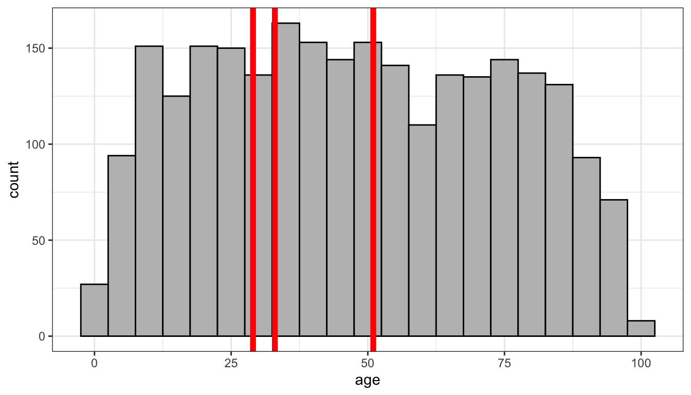

Figure 10: Histogram of Tomato Meter ratings from politics dataset with three candidates for the mode drawn in red

Interestingly, while it does not make sense to think about a mean or a median for quantitative variables, we can use the idea of the mode for categorical variables. The most common category is often referred to as the modal category. If you want to quickly identify the modal category for a categorical variable, you can wrap a table command inside a sort command with the decreasing=TRUE argument to see the top category at the right.

sort(table(movies$Rating), decreasing = TRUE)

## 
##     R PG-13    PG     G 
##  1143   991   363    56

R-Rated movies are the modal category for maturity rating in our movies dataset.

Comparing the mean and median

How can the mean and median give different results? Remember that the mean defines the balancing point and the median defines the midpoint. If you have a perfectly symmetric distribution, then these two points are the same because you would balance the distribution at the midpoint. However, when the distribution is skewed in one direction or another, the mean and the median will be different. In order to maintain balance, the mean will be pulled in the direction of the skew. When you have heavily skewed distributions, this can lead to dramatically different values for the mean and median.

Lets look at this phenomenon for a couple of variables in the movie dataset. As the histogram above showed, the Tomato Meter variable is fairly symmetric and as a result we end up with a mean (47.8) and median (47) that are pretty close. Figure 11 shows the distribution of movie runtime which is somewhat more right-skewed.

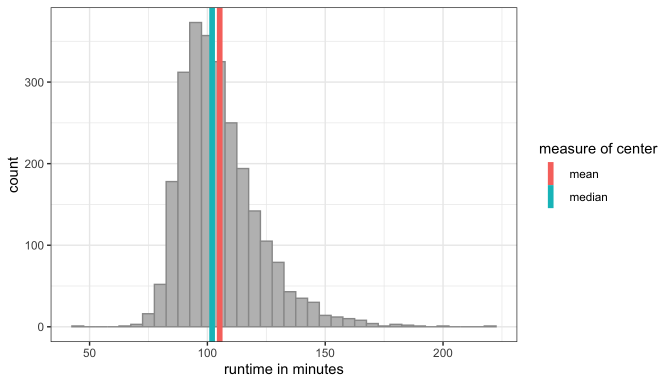
Figure 11: Distribution of movie runtime with mean (105.2) and median (102) shown as vertical lines

The skew here is not too dramatic, but it pulls the mean about 3 minutes higher than the median.

Figure 12 shows the distribution of box office returns to movies which is heavily right skewed. Most movies make moderate amounts of money, and then there are a few star performers that make bucket loads of cash.

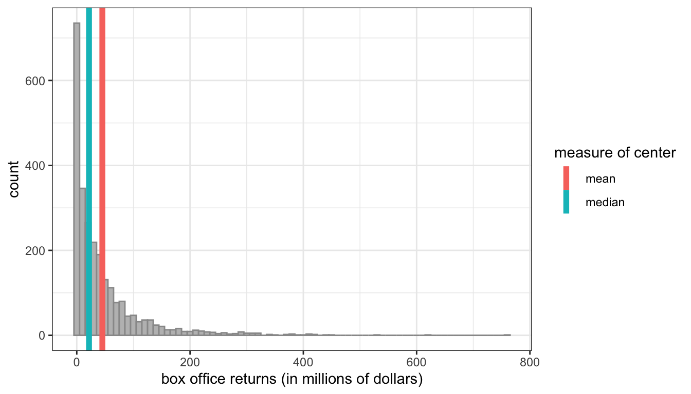
Figure 12: Distribution of movie box office returns with mean (45.2) and median (21.6) shown as vertical lines

As a result of this skew, the mean box office returns are about $45.2 million, while the median box office returns are about $21.6 million. The mean here is more than double the median!

Note that neither estimate is in some fundamental way incorrect. They are both correctly estimating what they were intended to estimate. It is up to us to understand and interpret these numbers correctly and to understand their limitations.

In many cases, we are actually more interested in the median as a measure of “average” experience than the mean, even though we think of the mean as the “average.” This is, for example, why you see home prices in an area always reported in terms of medians rather than means. Mean home prices tend to be much higher than median home prices because of the relatively few very expensive homes in a given area.