The Problem of Statistical Inference
So far, we have only been looking at measurements from our actual datasets. We examined both univariate statistics like the mean, median, and standard deviation, as well as measures of association like the mean difference, correlation coefficient and OLS regression line slope. We can use this measures to draw conclusions about our data.
In many cases, the dataset that we are working is only a sample from some larger population. Importantly, we don’t just want to know something about the sample, but rather we want to know something about the population from which the sample was drawn. For example, when polling organizations like Gallup conduct political polls of 500 people, they are not drawing conclusions about just those 500 people, but rather about the whole population from which those 500 people were sampled.
To take another example from our General Social Survey (GSS) data on sexual frequency. We can calculate the mean sexual frequency by marital status:
##       Married       Widowed      Divorced     Separated Never married
##     56.094106      9.222628     41.388720     55.652778     53.617704
Married respondents had sex 2.5 (56.1-53.6) times more per year than never married individuals. We don’t want to draw this conclusion just for our sample. Rather, we want to know what the relationship is between marital status and sexual frequency in the US population as a whole. In other words, we want to infer from our sample to the population. Figure 33 shows this process graphically.
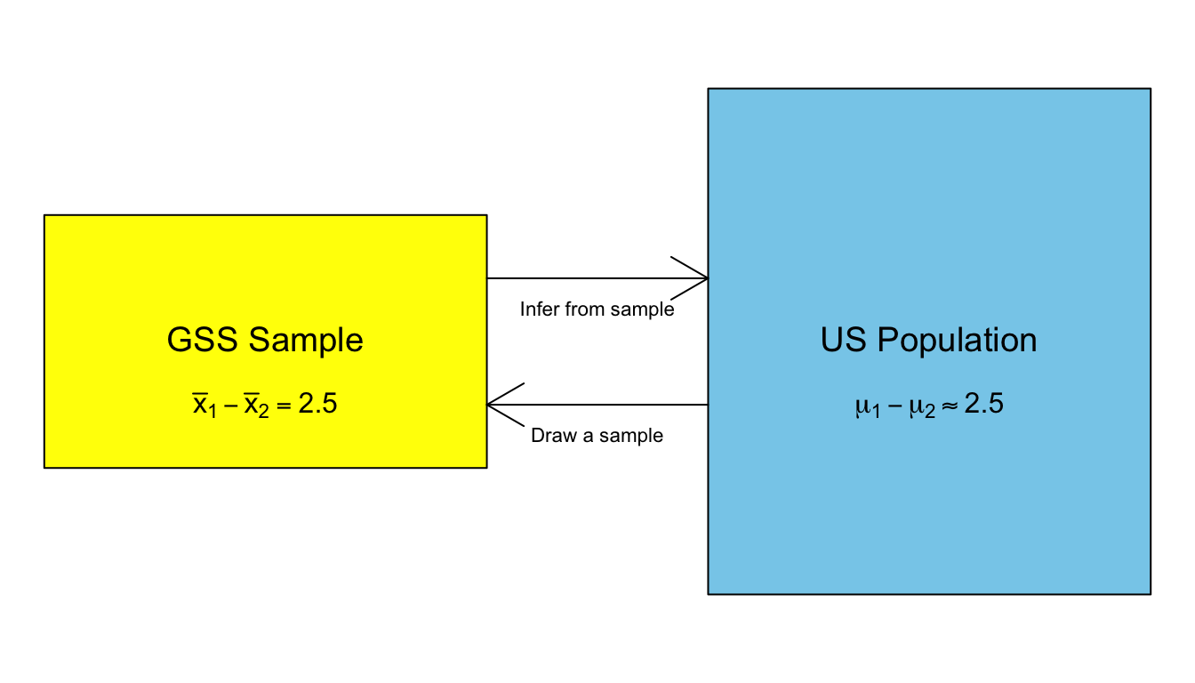
Figure 33: The process of making statistical inferences
The large blue rectangle is the population that we want to know about. Within this population, there is some value that we want to know. In this case, that value is the mean difference in sexual frequency between married and never married individuals. We refer to this unknown value in the population as a parameter. You will also notice that there are some funny-looking Greek letters in that box. We always use Greek symbols to represent values in the population. In this case, \(\mu_1\) is the population mean of sexual frequency for married individuals and \(\mu_2\) is the population mean of sexual frequency for never married individuals. Thus, \(\mu_1-\mu_2\) is the population mean difference in sexual frequency between married and never married individuals.
We typically don’t have data on the entire population, which is why we need to draw a sample in the first place. Therefore, these population parameters are unknown. To estimate what they are, we draw a sample as shown by the smaller yellow square. In this sample, we can calculate the sample mean difference in sexual frequency between married and never married individuals, \(\bar{x}_1-\bar{x}_2\). We refer to a measurement in the sample as a statistic. We represent these statistics with roman letters to distinguish them from the corresponding value in the population.
The statistic is always an estimate of the parameter. In this case, \(\bar{x}_1-\bar{x}_2\) is an estimate of \(\mu_1-\mu_2\). We can infer from the sample to the population and conclude that our best guess as to the true mean difference in the population is the value we got in the sample.
The sample mean difference may be our best guess as to the true value in the population, but how confident are we in that guess? Intuitively, if I only had a sample of 10 people I would be much less confident than if I had a sample of 10,000 people. Statistical inference is the technique of quantifying our uncertainty in the estimate. If you have ever read the results of a political poll, you will be familiar with the term “margin of error.” This is a measure of statistical inference.
Why might our sample produce inaccurate results? There are two sources of bias that could result in our sample statistic being different from the true population parameter. The first form of bias is systematic bias. Systematic bias occurs when something about the procedure for generating the sample produces a systematic difference between the sample and the population. Sometimes, systematic bias results from the way the sample is drawn. For example, if I sample my friends and colleagues on their voting behavior, I will likely introduce very large systematic bias in my estimate of who will win an election because my friends and colleagues are more likely than the general population to hold similar views to my own. Systematic bias can also result from the way questions are worded, the characteristics of interviewers, the time of day interviews are conducted, etc. Systematic bias can often be minimized in well-designed and executed scientific surveys. Statistical inference cannot do anything to account for systematic bias.
The second form of bias is random bias. Random bias occurs when the sample statistic is different from the population parameter, just by random chance due to the actual sample that was drawn. In other words, even if there is no systematic bias in my survey design, I can get a bad estimate simply due to the bad luck of drawing a really unusual sample. Imagine that I am interested in estimating mean wealth in the United States and I happen to draw Bill Gates in my sample. I will dramatically overestimate mean wealth in the US. Random bias affects every sample, regardless of how well-designed and executed.
In practice, the sample statistic is extremely unlikely to be exactly equal to the population parameter, so some degree of random bias is always present in every sample. However, this random bias will become less important as the sample size increases. In the previous example, Bill Gates is going to bias my results much more if I draw a sample of 10 people, than if I draw a sample of 100,000 people. Our goal with statistical inference is to more precisely quantify how bad that random bias could be in our sample.
Notice the word “could” in the previous sentence. The tricky part about statistical inference is that while we know that random bias could be causing our sample statistic to be very different from the population parameter, we never know for sure whether random bias had a big effect or a small effect in our particular sample, because we don’t have the population parameter with which we could compare it. Keep this issue in mind in the next sections, as it plays a key role in how we understand our procedures of statistical inference.
It is also important to keep in mind that statistical inference only works when you are actually drawing a sample from a larger population that you want to draw conclusions about. In some cases, our data either constitute a unique event, as in the Titanic case, that cannot be properly considered a sample of something larger or the data actually constitute the entire population of interest, as is the case in our dataset on movies. Although you will occasionally still see people use inferential measures on such data, it is technically inappropriate because there is no larger population to make inferences about.