Sample Design and Weighting
Thus far, we have acted as if all of the data we have analyzed comes from a simple random sample , or an SRS for short. For a sample to be a simple random sample, it must exhibit the following property:
In a simple random random sample (SRS) of size \(n\), every possible combination of observations from the population must have an equally likely chance of being drawn.
if every possible combination of observations from the population has an equally likely chance of being drawn, then every observation also has an equally likely chance of being drawn. This latter property is important. If each observation from the population has an equally likely chance to be drawn, then any statistic we draw from the sample should be unbiased - it should approximate the population parameter except for random bias. In simple terms, our sample should be representative of the population.
However, SRS’s have an additional criteria above and beyond each observation having an equally likely chance of being drawn. Every possible combination of observations from the population must have an equally likely chance of being drawn. What does this mean? Imagine that I wanted to sample two students from our classroom. First I divide the class into two equally sized groups and then I sample one student from each group. In this case, each student has an equal likelihood of being drawn, specifically \(2/N\) where \(N\) is the number of students in the class. However, not every possible combination of two students from the class is possible. Students will never be drawn in combination with another student from their own cluster.
This additional criteria for an SRS is necessary for the standard errors that we have been using to be accurate for measures of statistical inference such as hypothesis tests and confidence intervals. If this criteria is not true, then we must make adjustments to our standard errors to account for the sample design. These adjustments will typically lead to larger standarde errors.
In practice, due to issues of cost and efficiency, most large scale samples are not simple random samples and we must take into account these issues of sample design. In addition, samples sometimes intentionally oversample some groups (typically small groups in the population) and thus statustical results must be weighted in order to calculate unbiased statistics.
Cluster/multistage sampling
Cluster or multistage sampling is a sampling technique often used to reduce the time and costs of surveying. When surveys are conducted over a large area such as the entire United States, simple random samples are not cost effective. Surveyors would have to travel extensively across every region of the United States to interview respondents chosen for the sample. Therefore, in practice most surveys use some form of multistage sampling, which is a particular form of cluster sampling.
The idea of multistage sampling is that observations are first grouped into primary sampling units or PSUs. These PSUs are typically defined geographically. For example, the General Social Survey uses PSUs that are made up of a combination of metropolitan areas and clusters of rural counties. In the first stage of this sampling process, certain PSUs are sampled. Then at the second stage, individual observations are sampled within the PSUs. PSUs of unequal size are typically sampled relative to population size so that each observation still has an equally likely chance of being drawn.
In practice, there may be even more than two stages of sampling. For example, one might sample a counties as the PSU and then within sample counties may sample census tracts or blocks, before then sampling households within those tracts. A sample of schoolchildren might first sample school districts, and then schools within the district before sampling individual students.
If PSUs are sample with correct probability, then the resulting sample will still be representative because every observation in the population had an equally likely chance of being drawn. However, it will clearly violate the assumption of an SRS. The consequence of cluster sampling is that if the variable of interest is distributed differently across clusters, the resulting standard error for statistical inference will be greater than that calculated in our default formulas.
To see why this happens, lets take a fairly straightforward example: what percent of the US population is Mormon? The General Social Survey (GSS) collects information on religious affiliation, so this should be a fairly straightforward calculation. To do this I have extracted a subset of GSS data from 1972-2014 that includes religious affiliation. For reasons that will be explained in more detail in the next section, religious affiliation is divided into three categories and the Mormon affiliation is in the “other” variable. Taking account of some missing value issues, I can calculate the percent mormon by year:
relig$mormon <- ifelse(is.na(relig$relig), NA,
                       ifelse(!is.na(relig$other) &
                                relig$other=="mormon", TRUE,
                              FALSE))
mormons <- tapply(relig$mormon, relig$year, mean, na.rm=TRUE)
mormons <- data.frame(year=as.numeric(rownames(mormons)),
                      proportion=mormons,
                      n=as.numeric(table(relig$year)))
rownames(mormons) <- NULL
head(mormons)
## year proportion n
## 1 1972 0.009299442 1613
## 2 1973 0.003989362 1504
## 3 1974 0.005390836 1484
## 4 1975 0.006711409 1490
## 5 1976 0.006004003 1499
## 6 1977 0.007189542 1530Lets go ahead and plot this proportion up over time.
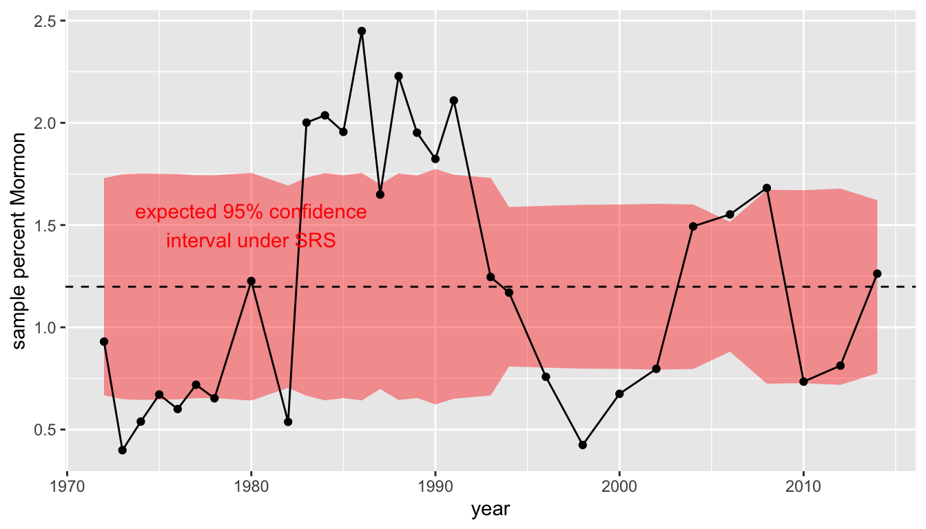
Figure 80: Sample percent Mormon over time from the General Social Survey, with a red band indicating expected 95% confidence intervals under assumption of SRS
In addition to the time series, I have included two other features. The dotted line gives the mean proportion across all years (1.19%). The red band gives the expected 95% confidence interval for sampling assuming that the mean across all years is correct and this proportion hasn’t changed over time. For each year this is given by:
\[0.0119 \pm 1.96(\sqrt{0.0119(1-0.0119)/n})\]
Where \(n\) is the sample size in that year.
What should be clear from this graph is that the actual variation in the sample proportion far exceeds that expected by simple random sampling. We would expect 19 out of 20 sample proportions to fall within that red band and most within the red band to fall close to the dotted line, but most values fall either outside the band or at its very edge. Our sample estimate of the percent Mormon fluctuates drastically from year to year.
Why do we have such large variation. The GSS uses geographically based cluster sampling and Mormons are not evenly distributed across the US. They are highly clustered in a few states (e.g. Utah, Idaho, Colorado, Nevada) and more commo in the western US than elsewhere. Therefore, in years where a Mormon PSU makes it into the sample we get overestimates of the percent Mormon and in years where a Mormon PSU does not make it into the sample, we get underestimates. Over the long term (assuming no change over time in the population) the average across years should give us an unbiased estimate of around 1.19%.
Stratification
In a stratified sample, we split our population into various strata by some characteristic and then sample observations from every stratum. For example, I might split households by household income strata of $25K. I would then sample observations from every single one of those income stratum.
On the surface, stratified sampling sounds very similar to clustering sample, but it has one important difference. In cluster/multistage sampling, only certain clusters are sampled. In stratified sampling, observations are drawn from all stratum. The goal is not cost savings or efficiency but ensuring adequate coverage in the final dataset for some variable of interest.
Stratified sampling also often has the opposite effect as clustered sampling. Greater similarity in some variable of interest within strata will actually reduce standard errors below that expected for simple random sampling, whereas greater similarity in some variable of interest in clusters will increase standard errors.
Observations can be drawn from stratum relative to population size in order to maintain the representativeness of the sample. However, researchers often intentionally sample some stratum with a higher frequency than their population size in order to ensure that small groups are present in enough size in the sample that representative statistics can be drawn for that group and comparisons can be made to other groups. For example, it is often common to oversample racial minorities in samples to ensure adequate inferences can be made for smaller groups. This is called oversampling.
If certain strata/groups are oversampled, then the sample will no longer be representative without applying some kind of weight. This leads us into a discussion of the issue of weights in sample design.
Weights
The use of weights in sample design can get quite complex and we will only scratch the surface here. The basic idea is that if your sample is not representative, you need to adjust all statistical results a sampling weight for each observation. The sampling weight for each observation should be equal to the inverse of that observation’s probability of being sampled \(p_i\). So:
\[w_i=\frac{1}{p_i}\]
To illustrate this, lets create a fictional population and draw a sample from it. For this exercise, I want to sample from the Dr. Seuss town of Sneetchville. There are two kinds of Sneetches in Sneetchville, those with stars on their bellies (Star-Bellied Sneetches) and regular Sneetches. Star-bellied Sneetches are relatively more advantaged and make up only 10% of the population. Lets create our populations by sampling incomes from the normal distribution.
reg_sneetch <- rnorm(18000, 10, 2)
sb_sneetch <- rnorm(2000, 15, 2)
sneetchville <- data.frame(type=factor(c(rep("regular",18000), rep("star-bellied",2000))),
                           income=c(reg_sneetch, sb_sneetch))
mean(sneetchville$income)
## [1] 10.47902## regular star-bellied
## 9.973621 15.027597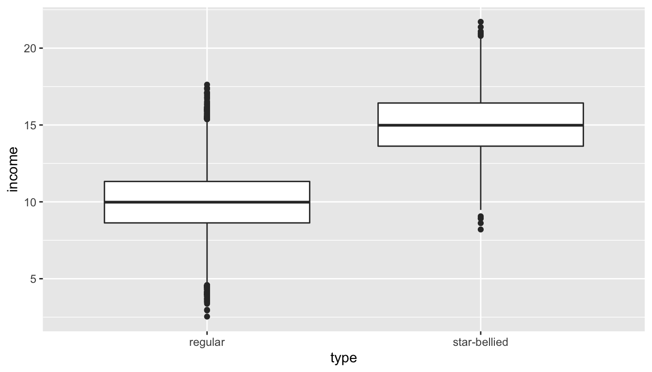
Figure 81: Distribution of income in Sneetchville by Sneetch type for the full population
We can see that Star-bellied Sneetches make considerably more than regular Sneetches on average. Because there are far more regular Sneetches, the mean income in Sneetchville of 10.5 is very close to the regular Sneetch mean income of 10.
Those are the population values which we get to see because we are omnipotent in this case. But our poor researcher needs to draw a sample to figure out these numbers. Lets say the researcher decides to draw a stratified sample that includes 100 of each type of Sneetch.
sneetch_sample <- sneetchville[c(sample(1:18000, 100, replace=FALSE),
                                 sample(18001:20000, 100, replace=FALSE)),]
mean(sneetch_sample$income)
## [1] 12.40761## regular star-bellied
## 10.02163 14.79360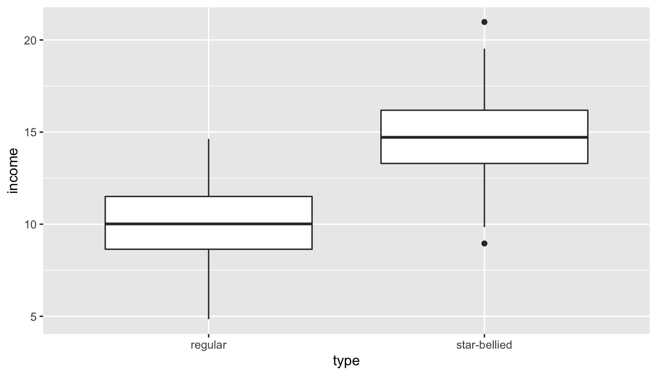
Figure 82: Distribution of income in Sneetchville by Sneetch type for statified sample
When I separate mean income by Sneetch type, I get estimates that are pretty close to the population values of 10 and 15. However, when I estimate mean income for the whole sample, I overestimate the population parameter substantially. It should be about 10.5 but I get 12.4. Why? My sample contains equal numbers of Star-bellied and regular Sneetches, but Star-bellied Sneetches are only about 10% of the population. Star-bellied Sneetches are thus over-represented and since they have higher incomes on average, I systematically overestimate income for Sneetchville as a whole.
I can correct for this problem if I apply weights that are equal to the inverse of the probability of being drawn. There are 2000 Star-bellied Sneetches in the population and I sampled 100, so the probability of being sampled is 100/2000. Similarly for regular Sneetches the probability is 100/18000.
sneetch_sample$sweight <- ifelse(sneetch_sample$type=="regular",
                                 18000/100, 2000/100)
tapply(sneetch_sample$sweight, sneetch_sample$type, mean)
## regular star-bellied
## 180 20The weights represent how many observations in the population a given observation in the sample represents. I can use these weights to get a weighted mean. A weighted mean can be calculated as:
\[\frac{\sum w_i*x_i}{\sum w_i}\]
## [1] 10.49883## [1] 10.49883Our weighted sample mean is now very close to the population mean of 10.5.
So why add this complication to my sample? Lets say I want to do a hypothesis test on the mean income difference between Star-bellied Sneetches and regular Sneetches in my sample. Lets calculate the standard error for that test:
## [1] 0.2974474Now instead of a stratified sample, lets draw a simple random sample of the same size (200) and calculate the same standard error.
sneetch_srs <- sneetchville[sample(1:20000,200, replace = FALSE),]
sqrt(sum((tapply(sneetch_srs$income, sneetch_srs$type, sd))^2/
  table(sneetch_srs$type)))
## [1] 0.5086267The standard errors on the mean difference are nearly doubled. Why? Remember that the sample size of each group is a factor in the standard error calculation. In this SRS we had the following:
##
##      regular star-bellied
##          182           18
We had far fewer Star-bellied Sneetches because we did not oversample them and this led to higher standard errors on any sort of comparison we try to draw between the two groups.
Post-stratification weighting
In some cases where oversamples are drawn for particular cases and population numbers are well known, it may be possible to calculate simple sample weights as we have done above. However, in many cases, researchers are less certain about how the sampling procedure itself might have under-represented or over-represented some groups. In these cases, it is common to construct post-stratification weights by comparing sample counts across a variety of strata to that from some trusted population source and then constructing weights that adjust for discrepancies. These kinds of calculations can be quite complex and we won’t go over them in detail here.
Weighting and standard errors
Regardless of how sample weights are constructed, they also have an effect on the variance in sampling. The use of sampling weights will increase the standard error of estimates above and beyond what we would expect in simple random sampling and this must be accounted for in statistical inference techniques. The greater the variation in sample weights, the bigger the design effect will be on standard errors.
Correcting for sample design in models
Clustering, stratification and weighting can all effect the representativeness and sampling variability of our sample. In samples that are not simple random samples, we need to take account of these design effects in our models.
To illustrate such design effects, we will consider the Add Health data that we have been using. This data is the result of a very complex sampling design. Schools were the PSU in a multistage sampling design. The school sample and the individual sample of students within schools were also stratified by a variety of characteristics. For example, the school sample was stratified by region of the US to ensure that all regions were represented. Certain ethnic/racial groups were also oversampled by design and post-stratification weights were also calculated.
In the publically available Add Health data, we do not have information on stratification variables, but we do have measures of clustering and weighting.
##   cluster   sweight
## 1     472 3663.6562
## 2     472 4471.7647
## 3     142 3325.3294
## 4     142  271.3590
## 5     145 3939.9402
## 6     145  759.0284
The cluster variable is a numeric id for each school and tells us which students were sampled from which PSU. The sweight variable is our sampling weight variable and tells us how many students in the US this observation represents.
Lets start with a naive model that ignores all of these design effects and just tries to predict number of friend nominations by our pseudoGPA measure:
##             Estimate Std. Error t value Pr(>|t|)
## (Intercept)    2.181      0.217  10.063        0
## pseudoGPA      0.837      0.074  11.304        0
This model is not necessarily representative of the population because it does not take account of the differential weight for each student. We can correct these estimates by adding in a weight argument to the lm command. This will essentially run a weighted least squares (WLS) model with these weights along the diagonal of the weight matrix. Intuitively, we are trying to minimize the weighted sum of squared residuals rather than the unweighted sum of squared residuals.
model_weighted <- lm(indegree~pseudoGPA, data=popularity, weights = sweight)
round(summary(model_weighted)$coef, 3)
## Estimate Std. Error t value Pr(>|t|)
## (Intercept) 2.267 0.220 10.312 0
## pseudoGPA 0.826 0.075 11.009 0In this case, the unweighted slope of 0.837 is not very differnet from the weighted slope of 0.826.
This model give us more representative and generalizable results, but we are still not taking account of the design effects that increase the standard errors of our estimates. Therefore, we are underestimating standard errors in the current model. There are two sources of these design effects that we need to account for:
- The variance in sample weights
- The cluster sampling
We can address the first issue of variance in sample weights by using robust standard errors:
library(sandwich)
library(lmtest)
model_robust <- coeftest(model_weighted, vcov=vcovHC(model_weighted, "HC1"))
model_robust
##
## t test of coefficients:
##
## Estimate Std. Error t value Pr(>|t|)
## (Intercept) 2.266634 0.268556 8.4401 < 2.2e-16 ***
## pseudoGPA 0.826424 0.094991 8.7001 < 2.2e-16 ***
## ---
## Signif. codes: 0 '***' 0.001 '**' 0.01 '*' 0.05 '.' 0.1 ' ' 1Notice that the standard error increased from about 0.075 to 0.095.
Robust standard errors will adequately address the design effect resulting from the variance of the sampling weights, but it does not address the design effect arising from clustering. Doing that is more mathematically complicated. We won’t go into the details here, but we will use the survey library in R that can account for a variety of design effects. To make use of this library, we first need to create a svydesign object that identifies the sampling design effects:
The survey library comes with a variety of functions that can be used to run a variety of models that expect this svydesign object rathre than a traditional data.frame. In this case, we want the svyglm command which can ge used to run “generalized linear models” which include our basic linear model.
##             Estimate Std. Error t value Pr(>|t|)
## (Intercept)    2.267      0.322   7.030        0
## pseudoGPA      0.826      0.109   7.593        0
We now get standard errors of about 0.109 which should reflect both the sampling weight heterogeneity and the cluster sampling design effects. Note that our point estimate of the slope is so large that even with this enlarged standard error, we are pretty confident the result is not zero.
| unweighted | weighted | robust SE | survey: weights | survey: weights+cluster | ||
|---|---|---|---|---|---|---|
| Intercept | 2.181*** | 2.267*** | 2.267*** | 2.267*** | 2.267*** | |
| (0.217) | (0.220) | (0.269) | (0.269) | (0.322) | ||
| GPA | 0.837*** | 0.826*** | 0.826*** | 0.826*** | 0.826*** | |
| (0.074) | (0.075) | (0.095) | (0.095) | (0.109) | ||
| R2 | 0.028 | 0.027 | ||||
| Num. obs. | 4397 | 4397 | 4397 | 4397 | ||
| p < 0.001; p < 0.01; p < 0.05 | ||||||
Table 18 shows all of the models estimated above plus an additional model that uses the survey library but only adjust for weights. All of the techniques except for the unweighted linear model produce identical and properly weighted estimates of the slope and intercept. They vary in the standard errors. The robust standard error approach produces results identical to the survey library method that only adjusts for weights. Only the final model using the survey library for weights and clustering addresses all of the design effects.