Missing Values
Up until this point, we have analyzed data that had no missing values. In actuality, the data did have missing values, but I used an imputation technique to remove the missing values to simplify our analyses. However, we now need to think more clearly about the consequences of missing values in datasets, because the reality is that most datasets that you want to use will have some missing data. Howe you handle this missing data can have important implications for your results.
Identifying Valid Skips
A missing value occurs when a value is missing for an observation on a particular value. Its important to distinguish in your data between situations in which a missing value is actually a valid response, from situations in which it is invalid and must be addressed.
It may seem unusual to think of some missing values as valid, but based on the structure of survey questionnaires is not unusual to run into valid missing values. In particular, valid skips are a common form of missing data. Valid skips occur when only a subset of respondents are asked a question that is a follow-up to a previous question. Typically to be asked the follow up question, respondents have to respond to the original question in a certain way. All respondents who weren’t asked the follow up question then have valid skips for their response.
As an example, lets look at how the General Social Survey asks about a person’s religious affiliation. The GSS asks this using a set of three questions. First, all respondents are asked “What is your religious preference? Is it Protestant, Catholic, Jewish, some other religion, or no religion?” After 1996, the GSS also started recording more specific responses for the “some other religion” category, but for simplicity lets just look at the distribution of this variable in 1996.
##
##   catholic     jewish       none      other protestant       <NA>
##        685         68        339        143       1664          5
On this variable, we have five cases of item nonresponse in which the respondent did not answer the question. They might have refused to answer it or perhaps they just did not know the answer.
For most of the respondents, this is the only question on religious affiliation. However, those who responded as Protestant are then asked further questions to determine more information about their particular denomination. This denom question includes prompts for most of the large denominations in the US. Here is the distribution of that variable.
##
##     afr meth ep zion   afr meth episcopal    am bapt ch in usa
##                    8                   11                   28
##      am baptist asso          am lutheran     baptist-dk which
##                   57                   51                  181
##            episcopal     evangelical luth   luth ch in america
##                   79                   33                   15
##    lutheran-dk which    lutheran-mo synod   methodist-dk which
##                   25                   48                   23
##  nat bapt conv of am    nat bapt conv usa      no denomination
##                   12                    8                   99
##                other       other baptists       other lutheran
##                  304                   69                   15
##      other methodist   other presbyterian presbyterian c in us
##                   12                   19                   34
##   presbyterian-dk wh presbyterian, merged     southern baptist
##                   11                   13                  273
##     united methodist united pres ch in us   wi evan luth synod
##                  190                   29                   11
##                 <NA>
##                 1246
Notice that we seem to have a lot of missing values here (1246). Did a lot of people just not know their denomination? No, in fact there is very little item nonresponse on this measure. The issue is that all of the people who were not asked this question because they didn’t respond as Protestant are listed as missing values here, but they are actually valid skips. We can see this more easily by crosstabbing the two variables based on whether the response was NA or not.
##
##              FALSE TRUE
##   catholic       0  685
##   jewish         0   68
##   none           0  339
##   other          0  143
##   protestant  1658    6
##   <NA>           0    5
You can see that almost all of the cases of NA here are respondents who did not identify as Protestants and therefore were not asked the denom question, i.e. valid skips. We have only six cases of individuals who were asked the denom question and did not respond.
For Protestants who did not identify with one of the large denominations prompted in denom were identified as “other”. For this group, a third question (called other in the GSS) was asked in which the respondent’s could provide any response. I won’t show the full table here as the number of denominations is quite large, but we can use the same logic as above to identify all of the valid skips vs. item nonresponses.
##
##                        FALSE TRUE
##   afr meth ep zion         0    8
##   afr meth episcopal       0   11
##   am bapt ch in usa        0   28
##   am baptist asso          0   57
##   am lutheran              0   51
##   baptist-dk which         0  181
##   episcopal                0   79
##   evangelical luth         0   33
##   luth ch in america       0   15
##   lutheran-dk which        0   25
##   lutheran-mo synod        0   48
##   methodist-dk which       0   23
##   nat bapt conv of am      0   12
##   nat bapt conv usa        0    8
##   no denomination          0   99
##   other                  300    4
##   other baptists           0   69
##   other lutheran           0   15
##   other methodist          0   12
##   other presbyterian       0   19
##   presbyterian c in us     0   34
##   presbyterian-dk wh       0   11
##   presbyterian, merged     0   13
##   southern baptist         0  273
##   united methodist         0  190
##   united pres ch in us     0   29
##   wi evan luth synod       0   11
##   <NA>                     0 1246
We can see here that of the individuals who identified with an “other” Protestant denomination, only four of those respondents did not provide a write-in response.
Valid skips are generally not a problem so long as we take account of them when we construct our final variable. In this example, we ultimately would want to use these three questions to create a parsimonious religious affiliation variable, perhaps by separating Protestants into evangelical and “mainline” denominations. In that case, the only item nonresponses will be the five cases for relig, the six cases for denom, and the four cases for other for a total of 15 real missing values.
Kinds of Missingness
In statistics, missingness is actually a word. It describes how we think values came to be missing from the data. In particular, we are concerned with whether missingness might be related to other variables that are related to the things we want to study. In this case, our results might be biased as a result of missing values. For example, income is a variable that often has lots of missing data. If missingness on income is related to education, gender, or race, then we might be concerned about how representative our results are in understanding the process. The biases that results from relationships between missingness and other variables can be hard to understand and therefore particularly challenging.
Missingness is generally considered as one of three types. The best case scenario is that the data are missing completely at random (MCAR). A variable is MCAR if every observation has the same probability of missingness. In other words, the missingness of a variable has no relationship to other observed or unobserved variables. If this is true, then removing observations with missing values will not bias results. However, it pretty rare that MCAR is a reasonable assumption for missingness. Perhaps if you randomly spill coffee on a page of your data, you might have MCAR.
A somewhat more realistic assumption is that the data are **missing at random* (MAR). Its totally obvious how this is different, right? A variable is MAR if the different probabilities of missingness can be fully accounted for by other observed variables in the dataset. If this is true, then various techniques can be used to produce unbiased results by imputing values for the missing values.
A more honest assessment is that the data are not missing at random (NMAR). A variable is NMAR if the different probabilities of missingness depend both on observed and unobserved variables. For example, some respondents may not provide income data because they are just naturally more suspicious. This variation in suspiciousness among respondents is not likely to be observed directly even though it may be partially correlated with other observed variables. The key issue here is the unobserved nature of some of the variables that produce missingness. Because they are unobserved, I have no way to account for them in my corrections. Therefore, I can never be certain that bias from missing values has been removed from my results.
In practice, although NMAR is probably the norm in most datasets, the number of missing values on a single variable may be small enough that even the incorrect assumption of MAR or MCAR might have little effect on the results. In my previous example, I had only 16 missing values on religious affiliation for 2904 respondents. So, its not likely to have a large effect on the results no matter how I deal with the missing values.
How exactly does one deal with those missing values? The data analyst typically has two choices. You can either remove cases with missing values or you can do some form of imputation. These two techniques are tied to the assumptions above. Removing cases is equivalent to assuming MCAR while imputation is equivalent to MAR.
To illustrate these different approaches below, we will look at a new example. We are going to examine the Add Health data again, but this time I am going to use a dataset that does not have imputed values for missing values. In particular, we are going to look at the relationship between parental income and popularity. Lets look at how many missing values we have for income.
##    Min. 1st Qu.  Median    Mean 3rd Qu.    Max.    NA's
##    0.00   23.00   40.00   45.37   60.00  200.00    1027
Yikes! We are missing 1027 cases of parental income. That seems like a lot. Lets go ahead and calculate the percent of missing cases for all of the variables in our data.
temp <- round(apply(is.na(addhealth), 2, mean)*100, 2)
temp <- data.frame(variable=names(temp), percent_missing=temp)
rownames(temp) <- NULL
pander(as.data.frame(temp))| variable | percent_missing |
|---|---|
| indegree | 0 |
| race | 0.05 |
| sex | 0 |
| grade | 1.18 |
| pseudoGPA | 1.91 |
| honorsociety | 0 |
| alcoholuse | 0.66 |
| smoker | 0.93 |
| bandchoir | 0 |
| academicclub | 0 |
| nsports | 0 |
| parentinc | 23.36 |
| cluster | 0 |
| sweight | 0 |
For most variables, we only have a very small number of missing values, typically less than 1% of cases. however, for parental income we are missing values for nearly a quarter of respondents.
Removing Cases
The simplest approach to dealing with missing values is to just drop observations (cases) that have missing values. In R, this is what will either happen by default or if you give a function the argument na.rm=TRUE. For example, lets calculate the mean income in the Add Health data:
## [1] NAIf we don’t specify how R should handle the missing values, R will report back a missing value for many basic calculations like the mean, median, and standard deviation. In order to get the mean for observations with valid values of income, we need to include the na.rm=TRUE option:
## [1] 45.37389The lm command in R behaves a little differently. It will automatically drop any observations that are missing values on any of the variables in the model. Lets look at this for a model predicting popularity by parental income and number of sports played:
##
## Call:
## lm(formula = indegree ~ parentinc + nsports, data = addhealth)
##
## Residuals:
##     Min      1Q  Median      3Q     Max
## -6.7920 -2.6738 -0.7722  1.8585 22.2967
##
## Coefficients:
##             Estimate Std. Error t value Pr(>|t|)
## (Intercept) 3.526054   0.114310  30.846  < 2e-16 ***
## parentinc   0.012309   0.001884   6.534 7.39e-11 ***
## nsports     0.451061   0.048920   9.220  < 2e-16 ***
## ---
## Signif. codes:  0 '***' 0.001 '**' 0.01 '*' 0.05 '.' 0.1 ' ' 1
##
## Residual standard error: 3.652 on 3367 degrees of freedom
##   (1027 observations deleted due to missingness)
## Multiple R-squared:  0.04164,    Adjusted R-squared:  0.04107
## F-statistic: 73.14 on 2 and 3367 DF,  p-value: < 2.2e-16
Note the comment in parenthesis at the bottom that tells us we lost 1027 observations due to missingness.
This approach is easy to implement but comes at a significant cost to the actual analysis. First, removing cases is equivalent to assuming MCAR, which is a strong assumption. Second, since most cases that you will remove typically have valid values on most of their variables, you are throwing away a lot of valid information as well as reducing your sample size. For example, all 1027 observations that were dropped in the model above due to missing values on parental income had valid responses the variable on number of sports played. If you are using a lot of variables in your analysis, then even with moderate amounts of missingness, you may reduce your sample size substantially.
In situations where only a very small number of values are missing, then removing cases may be a reasonable strategy for reasons of practicality. For example, in the Add Health data, the race variable has missing values on two observations. Regardless of whether the assumption of MCAR is violated or not, the removal of two observations in a sample of 4,397 is highly unlikely to make much difference. Rather, than use more complicated techniques that are labor intensive, it probably makes much more sense remove them.
Two strategies are available when you remove cases. You can either do available-case analysis or complete-case analysis. Both strategies refer to how you treat missing values in an analysis which will include multiple measurements that may use different numbers of variables. The most obvious and frequent case here is when you run multiple nested models in which you include different number of variables. For example, lets say we want to predict a student’s popularity by in a series of nested models: - Model 1: predict popularity by number of sports played - Model 2: add smoking and drinking behavior as predictors model 1 - Model 3: add parental income as a predictor to model 2
In this case, my most complex model is model 3 and it includes five variables: popularity, number of sports played, smoking behavior, drinking behavior, and parental income. I need to consider carefully how I am going to go about removing cases.
Available-case analysis
In available-case analysis (also called pairwise deletion) observations are only removed for each particular component of the analysis (e.g. a model) in which they are used. This is what R will do by default when you run nested models because it will only remove cases if a variable in that particular model is missing.
model1.avail <- lm(indegree~nsports, data=addhealth)
model2.avail <- update(model1.avail, .~.+alcoholuse+smoker)
model3.avail <- update(model2.avail, .~.+parentinc)
As a sidenote, I am introducing a new function here called update that can be very useful for model building. The update function can be used on a model object to make some changes to it and then re-run it. In this case, I am changing the model formula, but you could also use it to change the data (useful for looking at subsets), add weights, etc. When you want to update the model formula, the syntax .~.+ will include all of the previous elements of the formula and then you can make additions. I am using it to build nested models without having to repeat the entire model syntax every time.
| Model 1 | Model 2 | Model 3 | ||
|---|---|---|---|---|
| (Intercept) | 3.997*** | 3.851*** | 3.391*** | |
| (0.072) | (0.079) | (0.120) | ||
| nsports | 0.504*** | 0.508*** | 0.454*** | |
| (0.043) | (0.043) | (0.049) | ||
| alcoholuseDrinker | 0.707*** | 0.663*** | ||
| (0.155) | (0.180) | |||
| smokerSmoker | 0.194 | 0.383* | ||
| (0.162) | (0.188) | |||
| parentinc | 0.012*** | |||
| (0.002) | ||||
| R2 | 0.031 | 0.037 | 0.048 | |
| Num. obs. | 4397 | 4343 | 3332 | |
| ***p < 0.001; **p < 0.01; *p < 0.05 | ||||
Table 19 shows the results of the nested models in table form. Pay particular attention to the change in the number of observations in each model. In the first model, there are no missing values on nsports or indegree so we have the full sample size of 4397. In model 2, we are missing a few values on drinking and smoking behavior, so the sample size drops to 4343. In Model 3, we are missing a large number of observations, so the sample size drops to 3332. We lose nearly a quarter of the data from Model 2 to Model 3.
The changing sample sizes across models make model comparisons extremely difficult. We don’t know if changes from model to model are driven by different combinations of independent variables or changes in sample size. Note for example that the effect of smoking on popularity almost doubles from Model 2 to Model 3. Was that change driven by the fact that we controlled for parental income or was it driven by the exclusion of nearly a quarter of the sample. We have no way of knowing.
For this reason, available-case analysis is generally not the best way to approach your analysis. You don’t want your sample sizes to be changing across models. There are a few special cases (I will discuss one in the next section) where it may be acceptable and sometimes it is just easier in the early exploratory phase of a project, but in general you should use complete-case analysis.
Complete-case analysis
In complete-case analysis (also called listwise deletion) you remove observations that are missing on any variables that you will use in the analysis even for some calculations that may not involve those variables. This techniques ensures that you are always working with the same sample throughout your analysis so any comparisons (e.g. across models) are not comparing apples and oranges.
In our example, I need to restrict my sample to only observations that have valid responses for all five of the variables that will be used in my most complex model. I can do this easily with the na.omit command which will remove any observation that is missing any value in a given dataset:
addhealth.complete <- na.omit(addhealth[,c("indegree","nsports","alcoholuse","smoker","parentinc")])
model1.complete <- lm(indegree~nsports, data=addhealth.complete)
model2.complete <- update(model1.complete, .~.+alcoholuse+smoker)
model3.complete <- update(model2.complete, .~.+parentinc)| Model 1 | Model 2 | Model 3 | ||
|---|---|---|---|---|
| (Intercept) | 4.051*** | 3.876*** | 3.391*** | |
| (0.085) | (0.091) | (0.120) | ||
| nsports | 0.490*** | 0.494*** | 0.454*** | |
| (0.049) | (0.049) | (0.049) | ||
| alcoholuseDrinker | 0.717*** | 0.663*** | ||
| (0.181) | (0.180) | |||
| smokerSmoker | 0.372* | 0.383* | ||
| (0.189) | (0.188) | |||
| parentinc | 0.012*** | |||
| (0.002) | ||||
| R2 | 0.029 | 0.037 | 0.048 | |
| Num. obs. | 3332 | 3332 | 3332 | |
| ***p < 0.001; **p < 0.01; *p < 0.05 | ||||
Table 20 shows the results for the models using complete-case analysis. Note that the sample size for each model is the same and is equivalent to that for the most complex model in the available-case analysis above.
It is now apparent that the change in the effect of smoking on popularity above was driven by the removal of cases and not the controls for parental income. I can see this because now that I have performed the same sample restriction on Model 2, I get a similar effect size for smoking. Its worth noting that this is not really a great thing, because it suggests that by dropping cases, I am biasing the sample in some way, but at least I can make consistent comparisons across models.
When only a small number of cases are missing, then complete-case analysis is a reasonable option that is practical and not labor intensive. For example, I wouldn’t worry too much about the 54 cases lost due to the inclusion of smoking and drinking behavior in the models above. However, when you are missing substantial numbers of cases, either from a single variable or from the cumulative effects of dropping a moderate number of observations for lots of variables, then both case removal techniques are suspect. In those cases, it is almost certainly better to move to an imputation strategy.
Imputation
Imputing a “fake” value for a missing value may seem worse than just removing it, but in many cases imputation is a better alternative than removing cases. First, imputation allows us to preserve the original sample size as well as all of the non-missing data that would be thrown way for cases with some missing values. Second, depending on methodology, imputation may move from a MCAR assumption to a MAR assumption.
There are a variety of imputation procedures, but they can generally be divided up along two dimensions. First, predictive imputations use information about other variables in the dataset to impute missing values, while non-predictive imputations do not. In most cases, predictive imputation uses some form of model structure to predict missing values. Predictive imputation moves the assumption on missingness from MCAR to MAR, but is more complex (and thus prone to its own problems of model mis-specification) and more labor-intensive.
Second, random imputations include some randomness in the imputation procedure, while deterministic imputations do not include randomness. Including randomness is necessary in order to preserve the actual variance in the variable that is being imputed. Deterministic imputations will always decrease this variance and thus lead to under-estimation of inferential statistics. However, random imputation identify an additional issue because random imputations will produce slightly different results each time the imputation procedure is conducted. To be accurate, the researcher must account for this additional imputation variabilty in their results.
In general, the gold standard for imputation is called multiple imputation which is a predictive imputation that include randomness and adjusts for imputation variability. However, this technique is also complex and labor-intensive, so it may not be the best practical choice when the number of missing values is small. Below, I outline several of these different approaches, from simplest to most complex.
Non-predictive imputation
The simplest form of imputation is to just replace missing values with a single value. Since the mean is considered the “best guess” for the non-missing cases, it is customary to impute the mean value here and so this technique is generally called mean imputation. We can perform mean imputation in R simply by using the bracket-and-boolean approach to identify and replace missing values:
addhealth$parentinc.meani <- addhealth$parentinc
addhealth$incmiss <- is.na(addhealth$parentinc)
addhealth$parentinc.meani[addhealth$incmiss] <- mean(addhealth$parentinc, na.rm=TRUE)
I create a separate variable called parentinc.meani for the mean imputation so that I can compare it to other imputation procedures later. I also create an incmiss variable that is just a boolean indicating whether income is missing for a given respondent.
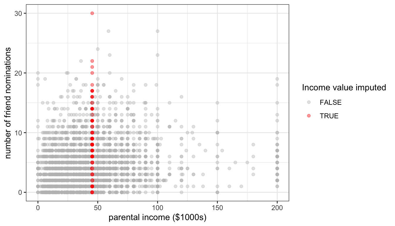
Figure 83: The effect of mean imputation of parental income on the scatterplot between parental income and number of friend nominations
Figure 83 shows the effect of mean imputation on the scatterplot of the relationship between parental income and number of friend nominations. All of the imputed values fall along a vertical line that corresponds to the mean parental income for the non-missing values. The effect on the variance of parental income is clear. Because this imputation procedure fits a single value, its imputation does not match the spread of observations along parental income. We can also see this by comparing the standard deviations of the original variable and the mean imputed one:
## [1] 33.6985## [1] 29.50069Since the variance of the independent variable is a component of the standard error calculation (see the first section of this chapter for details), underestimating the variance will lead to underestimates of the standard error in the linear model. A similar method that will account for the variance in the independent variable is to just randomly sample values of parental income from the valid responses. I can do this in R using the sample function.
addhealth$parentinc.randi <- addhealth$parentinc
addhealth$parentinc.randi[addhealth$incmiss]<-sample(addhealth$parentinc[!addhealth$incmiss],
                                                     sum(addhealth$incmiss),
                                                     replace = TRUE)
I create a new variable for this imputation. The sample function will sample from a given data vector (in this case the valid responses to parental income) a specified number of times (in this case the number of missing values). I also specify that I want to sample with replacement, which means that I replace values that I have already sampled before drawing a new value.
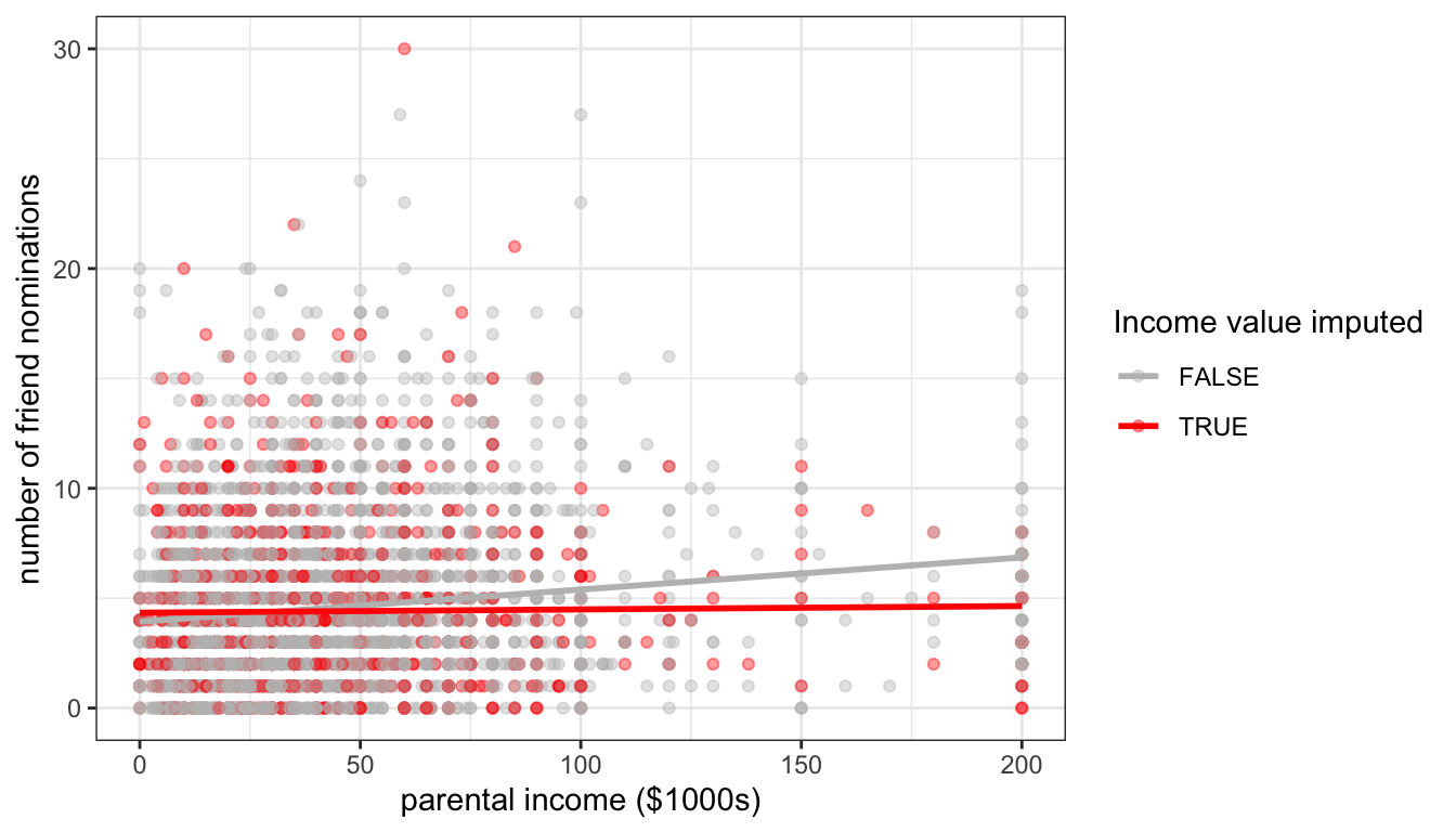
Figure 84: The effect of random imputation of parental income on the scatterplot between parental income and number of friend nominations
Figure 84 shows the same scatterplot as above, but this time with random imputation. You can see that my imputed values are now spread out across the range of parental income, thus preserving the variance in that variable.
Although random imputation is preferable to mean imputation, both methods have a serious drawback. Because I am imputing values without respect to any other variables, these imputed values will by definition be uncorrelated with the dependent variable. You can see this in figure 84 where I have drawn the best fitting line for the imputed and non-imputed values. The red line for the imputed values is basically flat because there will be no association except for that produced by sampling variability. Because imputed values are determined without any prediction, non-predictive imputation will always bias estimates of association between variables downward.
| sample | correlation | slope | sd |
|---|---|---|---|
| Valid cases | 0.132 | 0.0146 | 33.7 |
| Valid cases + mean imputed | 0.117 | 0.0146 | 29.5 |
| Valid cases + random imputed | 0.105 | 0.0114 | 33.9 |
Table 21 compares measures of association and variance in the Add Health data for these two techniques to the same numbers when only valid cases are used. The reduction in correlation in the two imputed samples is apparent, relative to the case with only valid responses. The reduction in variance of parental income is also clear for the case of mean imputation. Interestingly, the mean imputation does not downwardly bias the measure of slope because the reduction in correlation is perfectly offset by the reduction in variance. However, this special feature only holds when there are no other independent variables in the model and is also probably best thought of as a case of two wrongs (errors) not making a right (correct measurement).
In general, because of these issues with downward bias, non-predictive imputation is not and advisable technique. However, in some cases it may be preferable as a “quick and dirty” method that is useful for initial exploratory analysis or because the number of missing cases is moderate. It may also be reasonable if the variable that needs to be imputed is intended to serve primarily as a control variable and inferences are not necessarily going to be drawn for this variable itself.
In these cases where non-predictive imputation serves as a quick and dirty method, one additional technique, which I call mean imputation with dummy is advisable. In this case, the researcher performs mean imputation as above but also includes the missingness boolean variable into the model specification as above. The effect of this dummy is to estimate a slope and intercept for the imputed variable that is unaffected by the imputation, while at the same time producing a measure of how far out mean imputation is off relative to where the model expects the missing cases to fall.
Since, we already have an incmiss dummy variable, we can implement this model very easily. Lets try it in a model that predicts number of friend nominations by parental income and number of sports played.
model.valid <- lm(indegree~parentinc+nsports, data=addhealth)
model.meani <- lm(indegree~parentinc.meani+nsports, data=addhealth)
model.mdummyi <- lm(indegree~parentinc.meani+nsports+incmiss, data=addhealth)| No imputation | Mean imputation | Mean imputation w/dummy | ||
|---|---|---|---|---|
| Parent income | 0.01231*** | |||
| (0.00188) | ||||
| Parent income, mean imputed | 0.01220*** | 0.01221*** | ||
| (0.00186) | (0.00186) | |||
| Number of sports played | 0.45106*** | 0.47134*** | 0.46945*** | |
| (0.04892) | (0.04292) | (0.04297) | ||
| Income missing dummy | -0.12163 | |||
| (0.12911) | ||||
| Intercept | 3.52605*** | 3.47950*** | 3.50954*** | |
| (0.11431) | (0.10678) | (0.11144) | ||
| R2 | 0.04164 | 0.03999 | 0.04018 | |
| Num. obs. | 3370 | 4397 | 4397 | |
| ***p < 0.001; **p < 0.01; *p < 0.05 | ||||
Table 22 shows the results of these models. In this case, the results are very similar. The coefficient on the income missing dummy basically tells us how far the average number of friend nominations was off for cases with income missing relative to what was predicted by the model. In this case, the model is telling us that with a mean imputation the predicted value of friend nominations for respondents with missing income data is 0.12 nominations higher than where it is in actuality. If we believe our model, this might suggest that the parental income of those with missing income is somewhat lower than those who are not missing, on average.
This quick and dirty method is often useful in practice, but keep in mind that it still has the same problems of underestimating variance and assuming MCAR. A far better solution would be to move to predictive imputation.
Predictive imputation
In a predictive imputation, we use other variables in the dataset to get predicted values for cases that are missing. In order to do this, an analyst must specify some sort of model to determine predicted values. A wide variety of models have been developed for this, but for this course, we will only discuss the simple case of using a linear model to predict missing values (sometimes called regression imputation).
In the case of the Add Health data, we have a variety of other variables that we can consider using to predict parental income including race, GPA, alcohol use, smoking, honor society membership, band/choir membership, academic club participation, and number of sports played. We also could consider using the dependent variable (number of friend nominations) here but there is some debate on whether dependent variables should be used to predict missing values, so we will not consider it here.
There is really no reason not to use as much information as possible here, so I will use all of these variables. However, in order to model this correctly, I want to consider the skewed nature of the my parental income data. To reduce the skewness and produce better predictions, I will transform parental income in my predictive model by square rooting it. I can then fit a model predicting parental income:
addhealth$parentinc.regi <- addhealth$parentinc
model <- lm(sqrt(parentinc)~race+pseudoGPA+honorsociety+alcoholuse+smoker
            +bandchoir+academicclub+nsports, data=addhealth)
predicted <- predict(model, addhealth)
addhealth$parentinc.regi[addhealth$incmiss] <- predicted[addhealth$incmiss]^2
summary(addhealth$parentinc.regi)
## Min. 1st Qu. Median Mean 3rd Qu. Max. NA's
## 0.00 25.19 39.83 43.87 54.20 200.00 39After fitting the model, I just use the predict command to get predicted parental income values (square rooted) for all of my observations. I remember to square these predicted values when I impute them back.
One important thing to note is that my imputed parental income still has 39 missing values. That is a lot less than 1027, but how come we didn’t remove all the missing values? The issue here is that some of my predictor variables (particularly smoking, alcohol use, and GPA) also have missing values. Therefore, for observations that are missing on those values as well as parental income, I will get missing values in my prediction. I will address how to handle this problem further below.
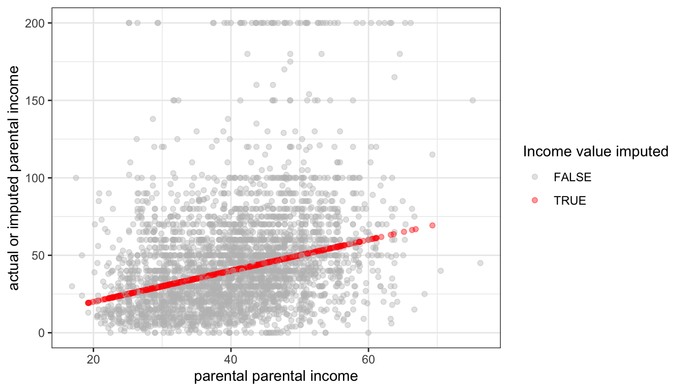
Figure 85: The relationship between predicted values of imputed parental income and actual or imputed values, using regression imputation
This regression imputation only accounts for variability in parental income that is accountable for in the model and ignores residual variation. This can be clearly seen in Figure 85 where the actual values of parental income are widely dispersed around the predicted values, except for cases where missing values were imputed. This imputation procedure therefore underestimates the total variance in parental income with similar consequences as above.
To address this problem, we can use random regression imputation which basically adds a random “tail” onto each predicted value based on the variance of our residual terms. It is also necessary to define a distribution from which to sample our random tails. We will use the normal distribution.
addhealth$parentinc.rregi <- addhealth$parentinc
model <- lm(sqrt(parentinc)~race+pseudoGPA+honorsociety+alcoholuse+smoker
            +bandchoir+academicclub+nsports, data=addhealth)
predicted <- predict(model, addhealth)
addhealth$parentinc.rregi[addhealth$incmiss] <- (predicted[addhealth$incmiss]+
                                                   rnorm(sum(addhealth$incmiss), 0, sigma(model)))^2
The rnorm function samples from a normal distribution with a given mean and standard deviation. We use the sigma function to pull the standard deviation of the residuals from our model.
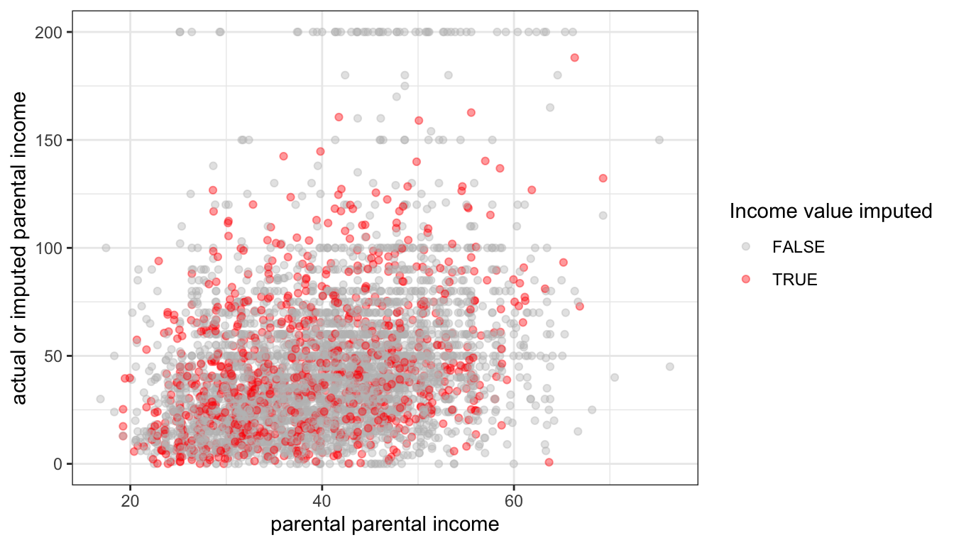
Figure 86: The relationship between predicted values of imputed parental income and actual or imputed values, using random regression imputation
Figure 86 shows that the variation of our imputed values now mimics that of the actual values. We can also compare the standard deviations across imputations to see that we have preserved the variation in our valid data:
## [1] 33.6985## [1] 30.10024## [1] 32.99728Chained equations
As we saw above, one downside of using a model to predict missing values is that missing values on other variables in the dataset can cause the imputation procedure to not impute all of the missing values. There are a few different ways of handling this but the most popular technique is to use an iterative procedure called **multiple imputation by chained equations* or MICE for short. The basic procedure is as follows:
- All missing values are given some placeholder value. This might be the mean value, for example.
- For one variable, the placeholder values are removed and missing values put back in. These missing values are then predicted and imputed by some model for this variable.
- Step 2 is repeated for all variables with missing values. When all variables have been imputed, we have completed one iteration.
- Steps 2-3 are then repeated again for some number of iterations. The number of iterations necessary may vary by data, but five iterations is typical.
The purpose of the iterations is to improve the imputation by moving further and further away from the mean imputation that was used to get an initial fit.
This procedure is complicated to implement in practice, but luckily the mice library in R already provides an excellent implementation. Furthermore, the mice library has a variety of modeling options that include the ability to handle missing values in both quantitative and categorical models. For quantitative variables, it does not by default use regression imputation, but rather a technique called predictive mean matching that is more flexible and resistant to mis-specification.
The basic command in the mice library to run MICE is … mice:
library(mice)
addhealth.complete <- mice(addhealth[,c("indegree","race","sex","grade","pseudoGPA",
                                        "honorsociety","alcoholuse","smoker","bandchoir",
                                        "academicclub","nsports","parentinc")], m=5)
##
## iter imp variable
## 1 1 race grade pseudoGPA alcoholuse smoker parentinc
## 1 2 race grade pseudoGPA alcoholuse smoker parentinc
## 1 3 race grade pseudoGPA alcoholuse smoker parentinc
## 1 4 race grade pseudoGPA alcoholuse smoker parentinc
## 1 5 race grade pseudoGPA alcoholuse smoker parentinc
## 2 1 race grade pseudoGPA alcoholuse smoker parentinc
## 2 2 race grade pseudoGPA alcoholuse smoker parentinc
## 2 3 race grade pseudoGPA alcoholuse smoker parentinc
## 2 4 race grade pseudoGPA alcoholuse smoker parentinc
## 2 5 race grade pseudoGPA alcoholuse smoker parentinc
## 3 1 race grade pseudoGPA alcoholuse smoker parentinc
## 3 2 race grade pseudoGPA alcoholuse smoker parentinc
## 3 3 race grade pseudoGPA alcoholuse smoker parentinc
## 3 4 race grade pseudoGPA alcoholuse smoker parentinc
## 3 5 race grade pseudoGPA alcoholuse smoker parentinc
## 4 1 race grade pseudoGPA alcoholuse smoker parentinc
## 4 2 race grade pseudoGPA alcoholuse smoker parentinc
## 4 3 race grade pseudoGPA alcoholuse smoker parentinc
## 4 4 race grade pseudoGPA alcoholuse smoker parentinc
## 4 5 race grade pseudoGPA alcoholuse smoker parentinc
## 5 1 race grade pseudoGPA alcoholuse smoker parentinc
## 5 2 race grade pseudoGPA alcoholuse smoker parentinc
## 5 3 race grade pseudoGPA alcoholuse smoker parentinc
## 5 4 race grade pseudoGPA alcoholuse smoker parentinc
## 5 5 race grade pseudoGPA alcoholuse smoker parentincIn this case, I specified all of the variables that I wanted to go into my multiple imputation. If you want all of the variables in your dataset to be used, you can just feed in the dataset with no list of variable names. You can see that mice went through five iterations of imputation, with a list of the variables imputed and the order in which they were imputed. You can also see that it cycled through something called “imp.” This value corresponds to the m=5 argument I specified. This is the number of times that mice performed the entire imputation procedure. In this case, I now have five complete datasets (datasets with no missing values) in the object addhealth.complete. To access any one of them, I need to use the complete function with an id number:
##     indegree                                    race          sex
##  Min.   : 0.000    White                          :2638   Length:4397
##  1st Qu.: 2.000    Black/African American         :1145   Class :character
##  Median : 4.000   Latino                          : 400   Mode  :character
##  Mean   : 4.551    Asian/Pacific Islander         : 161
##  3rd Qu.: 6.000    Other                          :  27
##  Max.   :30.000    American Indian/Native American:  26
##      grade          pseudoGPA     honorsociety          alcoholuse
##  Min.   : 7.000   Min.   :1.000   Mode :logical   Non-drinker:3669
##  1st Qu.: 8.000   1st Qu.:2.250   FALSE:3990      Drinker    : 728
##  Median :10.000   Median :3.000   TRUE :407
##  Mean   : 9.507   Mean   :2.832
##  3rd Qu.:11.000   3rd Qu.:3.500
##  Max.   :12.000   Max.   :4.000
##         smoker     bandchoir       academicclub       nsports
##  Non-smoker:3732   Mode :logical   Mode :logical   Min.   :0.000
##  Smoker    : 665   FALSE:3340      FALSE:3578      1st Qu.:0.000
##                    TRUE :1057      TRUE :819       Median :1.000
##                                                    Mean   :1.098
##                                                    3rd Qu.:2.000
##                                                    Max.   :6.000
##    parentinc
##  Min.   :  0.00
##  1st Qu.: 22.00
##  Median : 40.00
##  Mean   : 44.83
##  3rd Qu.: 60.00
##  Max.   :200.00
I can run a model on my first complete dataset like so:
##
## Call:
## lm(formula = indegree ~ parentinc, data = complete(addhealth.complete,
##     1))
##
## Residuals:
##     Min      1Q  Median      3Q     Max
## -6.0257 -2.6372 -0.7634  1.7695 25.0963
##
## Coefficients:
##             Estimate Std. Error t value Pr(>|t|)
## (Intercept) 3.921902   0.092148  42.561   <2e-16 ***
## parentinc   0.014026   0.001646   8.523   <2e-16 ***
## ---
## Signif. codes:  0 '***' 0.001 '**' 0.01 '*' 0.05 '.' 0.1 ' ' 1
##
## Residual standard error: 3.662 on 4395 degrees of freedom
## Multiple R-squared:  0.01626,    Adjusted R-squared:  0.01604
## F-statistic: 72.64 on 1 and 4395 DF,  p-value: < 2.2e-16
Addressing imputation variability
Why did I run five different imputations using the mice function in the example above? To explore this question, lets first look at the slope predicting the number of friend nominations by parental income across all five complete imputations:
coefs <- NULL
for(i in 1:5) {
  coefs <- c(coefs,
             coef(lm(indegree~parentinc, data=complete(addhealth.complete,i)))[2])
}
coefs
## parentinc parentinc parentinc parentinc parentinc
## 0.01402563 0.01459309 0.01415435 0.01400471 0.01483226I get different values on each complete imputation. This is because there is an element of randomness in my imputation procedure. That randomness is needed to correctly impute while preserving the variance in the underlying variables, but it adds an additional layer of uncertainty to understanding my results. Which of these values should I use for my results? This additional layer of uncertainty is called imputation variability. Imputation variability adds additional uncertainty above and beyond sampling variability when attempting to make statistical inferences.
To accurately account for imputation variability, we need to use multiple imputation. The multiple imputation process is as follows:
- Use imputation process with random component to impute missing values and repeat this process to produce m separate complete datasets. Each of these datasets will be somewhat different due to the randomization of imputation. Usually
m=5is sufficient. - Run
mseparate parallel models on each imputed dataset. As a result, you will havemsets of regression coefficients and standard errors. - Pool the regression coefficients across datasets by taking the mean across all
mdatasets. - Pool standard errors by taking the average standard errors across all
mdatasets plus the between model standard deviation in coefficients. The formula for the overall standard error is:
\[SE_{\beta}=\sqrt{W+B+\frac{B}{m}}\] Where \(W\) is the squared average standard error across all \(m\) datasets and \(B\) is the variance in coefficient estimates across all \(m\) models.
The mice library provides some nice utilities for accounting for multiple imputation in basic linear models. However, it is worth learning how to to do this procedure by hand, so I will first show you how to do it without using built-in functions.
The first step is to loop through each imputation, calculate the model and extract the coefficients and standard errors:
b <- se <- NULL
for(i in 1:5) {
  model <- lm(indegree~parentinc+smoker+alcoholuse+nsports,
              data=complete(addhealth.complete,i))
  b <- cbind(b, coef(model))
  se <- cbind(se, summary(model)$coef[,2])
}
The b and se objects are just matrices of the regression coefficients and standard errors across imputations. For example:
##                    [,1]  [,2]  [,3]  [,4]  [,5]
## (Intercept)       3.392 3.365 3.376 3.383 3.360
## parentinc         0.011 0.012 0.012 0.011 0.012
## smokerSmoker      0.227 0.210 0.203 0.214 0.181
## alcoholuseDrinker 0.599 0.620 0.640 0.624 0.630
## nsports           0.468 0.468 0.469 0.471 0.465
With the application of the apply command we can estimate averages for these values across imputations as well as the variability in regression coefficients across models.
b.pool <- apply(b,1,mean)
between.var <- apply(b,1,var)
within.var <- apply(se^2,1,mean)
se.pool <- sqrt(within.var+between.var+between.var/5)
t.pool <- b.pool/se.pool
pvalue.pool <- (1-pnorm(abs(t.pool)))*2
results <- data.frame(b.pool, se.pool, t.pool, pvalue.pool)
round(results,4)
## b.pool se.pool t.pool pvalue.pool
## (Intercept) 3.3751 0.1037 32.5503 0.0000
## parentinc 0.0118 0.0017 6.9758 0.0000
## smokerSmoker 0.2071 0.1604 1.2909 0.1967
## alcoholuseDrinker 0.6226 0.1546 4.0269 0.0001
## nsports 0.4681 0.0430 10.8793 0.0000We now have results that make use of a complete dataset and also adjust for imputation variability. We can also use the results above to estimate the relative share of the between and within variation to our total uncertainty. Figure 87 shows the relative contribution of between and within variability to our total uncertainty. Because most variables in this model are missing few or no values, the contribution of between sample imputation variability is quite small for most cases. However, for parental income which was missing a quarter of observations, it is a substantial share of around 30% of the total variability.
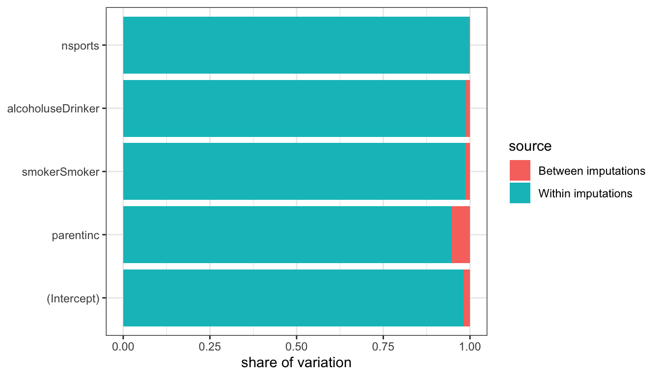
Figure 87: Share of variability for each estimated coefficient that comes from between sample imputation variability vs. within sample sampling variabilty
The for-loop approach above is an effective method for pooling results for multiple imputation and is flexible enough that you can utilize a wide variety of techniques within the for-loop, such as adjustments for sample design. However, if you are just running vanilla lm commands, then the mice library also has an easier approach:
model.mi <- pool(with(addhealth.complete, lm(indegree~parentinc+smoker+alcoholuse+nsports)))
summary(model.mi)
## estimate std.error statistic df p.value
## (Intercept) 3.37512372 0.103689400 32.550325 3182.639 0.000000e+00
## parentinc 0.01175002 0.001684391 6.975823 1090.345 5.265122e-12
## smokerSmoker 0.20712655 0.160449662 1.290913 3630.841 1.968160e-01
## alcoholuseDrinker 0.62262913 0.154619376 4.026851 3792.738 5.763470e-05
## nsports 0.46810932 0.043027384 10.879335 4337.942 0.000000e+00As I said earlier, multiple imputation is the gold standard for dealing with missing values. However, it is important to realize that it is not a bulletproof solution to the problem of missing values. It still assumes MAR and if the underlying models used to predict missing values are not good, then it may not produce the best results. Ideally, when doing any imputation procedure you should also perform an analysis of your imputation results to ensure that they are reasonable. These techniques are beyond the scope of this class, but further reading links can be found on Canvas.