The IID Violation and Robust Standard Errors
Lets return to the idea of the idea of the linear model as a data-generating process:
\[y_i=\underbrace{\beta_0+\beta_1x_{i1}+\beta_2x_{i2}+\ldots+\beta_px_{ip}}_{\hat{y}_i}+\epsilon_i\]
To get a given value of \(y_i\) for some observation \(i\) you feed in all of the independent variables for that obseravation into your linear model equation to get a predicted value, \(\hat{y}_i\). However, you still need to take account of the stochastic element that is not predicted by your linear function. To do this, imagine reaching into a bag full of numbers and pulling out one value. Thats your \(\epsilon_i\) which you add on to your predicted value to get the actual value of \(y\).
What exactly is in that “bag full of numbers?” Each time you reach into that bag, you are drawing a number from some distribution based on the values in that bag. The procedure of estimating linear models makes two key assumption about how this process works:
- Each observation is drawing from the same bag. In other words, you are drawing values from the same distribution. The shape of this distribution does not matter, even though some people will claim that it must be normally distributed. However, regardless of the shape, all obervations must be drawing from an identically shaped distribution.
- Each draw from the bag must be independent. This means that the value you get on one draw does not depend in any way on other draws.
Together these two assumptions are often called the IID assumption which stands for independent and identically distributed.
What is the consequence of violating the IID assumption? The good news is that violating this assumption will not bias your estimates of the slope and intercept. The bad news is that violating this assumption will often produce incorrect standard errors on your estimates. In the worst case, you may drastically underestimate standard errors and thus reach incorrect conclusions from classical statistical inference procedures such as hypothesis tests.
How do IID violations occur? Lets talk about a couple of common cases.
Violations of independence
The two most common ways for the independence assumption to be violated are by serial autocorrelation and repeated observations.
Serial autocorrelation
Serial autocorrelation occurs in longitudinal data, most commonly with time series data. In this case, observations close in time tend to be more similar for reasons not captured by the model and thus you observe a positive correlation between subsequent residuals when they are ordered by time.
For example, the longley data that come as an example dataset in base R provide a classic example of serial autocorrelation, as illustrated in Figure 77.
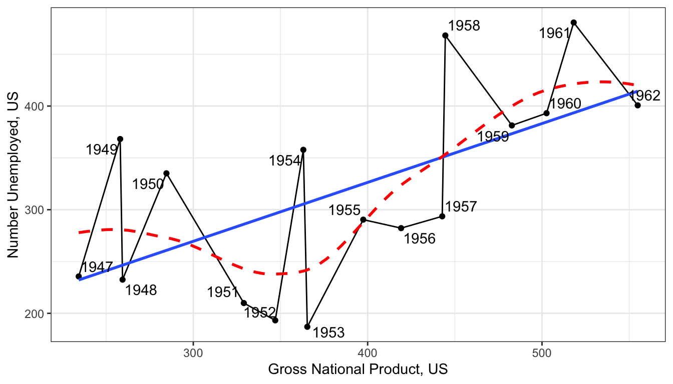
Figure 77: Scatterplot of GNP and number of workers unemployed, US 1947-1962
The number unemployed tends to be cyclical and cycles last longer than a year, so we get a an up-down-up pattern show in red that leads to non-independence among the residuals from the linear model (shown in blue).
We can more formally look at this by looking at the correlation between temporally-adjacent residuals, although this requires a bit of work to set up.
model <- lm(Employed~GNP, data=longley)
temp <- augment(model)$.resid
temp <- data.frame(earlier=temp[1:15], later=temp[2:16])
head(temp)
## earlier later
## 1 0.33732993 0.26276150
## 2 0.26276150 -0.64055835
## 3 -0.64055835 -0.54705800
## 4 -0.54705800 -0.05522581
## 5 -0.05522581 -0.26360117
## 6 -0.26360117 0.44744315The two values in the first row are the residuals fro 1947 and 1948. The second row contains the residuals for 1948 and 1949, and so on. Notice how the later value becomes the earlier value in the next row.
Lets look at how big the serial autocorrelation is:
## [1] 0.1622029We are definitely seeing some positive serial autocorrelation, but its of a moderate size in this case.
Repeated observations
Imagine that you have data on fourth grade students at a particular elementary school. You want to look at the relationship between scores on some test and a measure of socioeconomic status (SES). In this case, the students are clustered into different classrooms with different teachers. Any differences between classrooms and teachers that might affect test performance (e.g. quality of instruction, lower stugdent/teacher ratio, aid in class) will show up in the residual of your model. But because students are clustered into these classrooms, their residuals will not be independent. Students from a “good” classroom will tend to have higher than average residuals while students from a “bad” classroom will tend to have below average residuals.
The issue here is that our residual terms are clustered by some higher-level identification. This problem most often appears when your data have a multilevel structure in which you are drawing repeated observations from some higher-level unit.
Longitudinal or panel data in which the same respondent is interviewed at different time intervals inherently face this problem. In this case, you are drawing repeated observations on the same individual at different points in time and so you expect that if that respondent has a higher than average residual in time 1, they also likely have a higher than average residual in time 2. However, as in the classroom example above, it can occur in a variety of situations even with cross-sectional data.
Heteroscedasticity
Say what? Yes, this is a real term. Heteroscedasticity means that the variance of your residuals is not constant but depends in some way on the terms in your model. In this case, observations are not drawn from identical distributions because the variance of this distribution is different for different observations.
One of the most common ways that heteroscedasticity arises is when the variance of the residuals increases with the predicted value of the dependent variables. This can easily be diagnosed on a residual by fitted value plot, where it shows up as a cone shape as in Figure 78.
model <- lm(BoxOffice~Runtime, data=movies)
ggplot(augment(model), aes(x=.fitted, y=.resid))+
  geom_point(alpha=0.7)+
  scale_y_continuous(labels=scales::dollar)+
  scale_x_continuous(labels=scales::dollar)+
  geom_hline(yintercept = 0, linetype=2)+
  theme_bw()+
  labs(x="predicted box office returns",
       y="residuals from the model")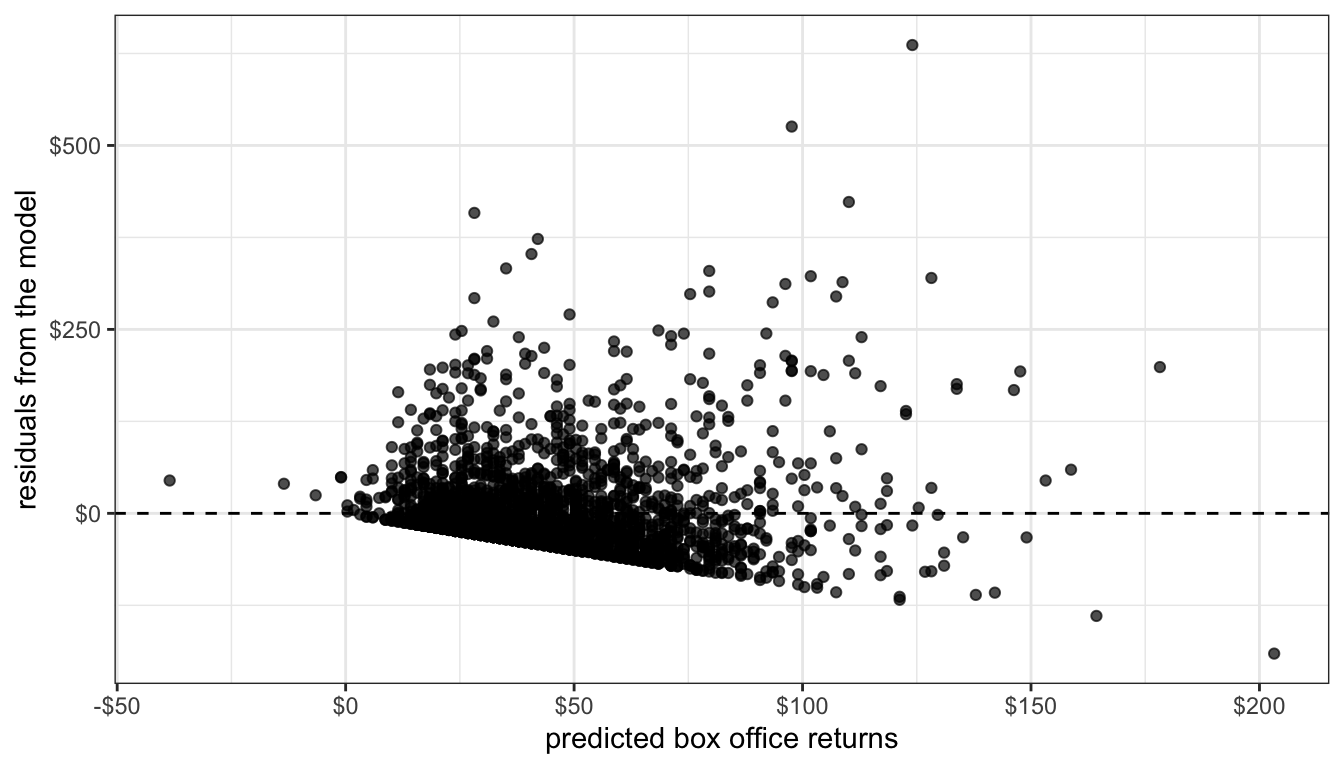
Figure 78: Residual plot of model predicting box office returns by movie runtime
Such patterns are common with right-skewed variables that have a lower threshold (often zero). In Figure 78, the residuals can never produce an actual value below zero, leading to the very clear linear pattern on the low end. The high end residuals are more scattered but also seem to show a cone pattern. Its not terribly surprising that as our predicted values grow in absolute terms, the residuals from this predicted value also grow in absolute value. In relative terms, the size of the residuals may be more constant.
Fixing IID violations
Given that you have identified an IID violation in your model, what can you do about it? The best solution is to get a better model. IID violations are often implicitly telling you that the model you have selected is not the best approach to the actual data-generating process that you have.
Lets take the case of heteroscedasticity. If you observe a cone shape to the residuals, it suggests that the absolute size of the residuals is growing with the size of the predicted value of your dependent variable. In relative terms (i.e. as a percentage of the predicted value), the size of those residuals may be more constant. A simple solution would be to log our dependent variable because this would move us from a model of absolute change in the dependent variable to one of relative change.
model <- lm(log(BoxOffice)~Runtime, data=movies)
ggplot(augment(model), aes(x=.fitted, y=.resid))+
  geom_point(alpha=0.7)+
  geom_hline(yintercept = 0, linetype=2)+
  theme_bw()+
  labs(x="predicted log of box office returns",
       y="residuals from the model")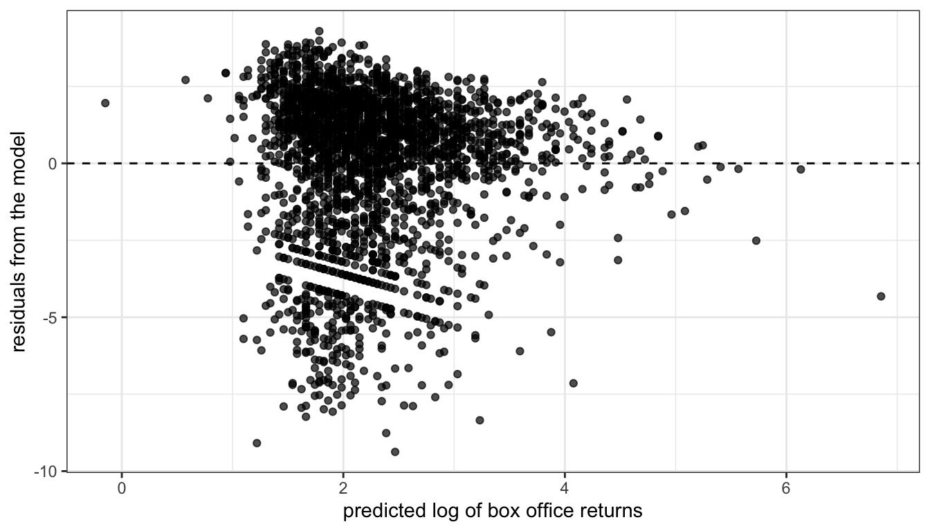
Figure 79: Residual plot of model predicting the log of box office returns by movie runtime
I now no longer observe the cone shape to my residuals. I might be a little concerned about the lack of residuals in the lower right quadrant, but overall this plot does not suggest a strong problem of heteroscedasticity. Furthermore, loggin box office returns may help address issues of non-linearity and outliers and give me results that are more sensible in terms of predicting percent change in box office returns rather than absolute dollars and cents.
Similarly, the problem of repeated observations can be addressed by the use of multilevel models that explicitly account for the higher-level units that repeated observations are clustered within. We won’t talk about these models in this course, but in aaddition to resolving the IID problem, these models make possible more interesting and complex models that analyze effects at different levels and across levels.
In some cases, a clear and better alternative may not be readily apparent. In this case, two techniques are common. The first is the use of weighted least squares and the second is the use of robust standard errors. Both of these techniques mathematically correct for the IID violation on the existing model. Weighted least squares requires the user to specify exacty how the IID violation arises, while robust standard errors seemingly figures it out mathemagically.
Weighted least squares
To do a weighted least squares regression model, we need to add a weighting matrix, \(\mathbf{W}\), to the standard matrix calculation of model coefficients and standard errors:
\[\mathbf{\beta}=(\mathbf{X'W^{-1}X})^{-1}\mathbf{X'W^{-1}y}\] \[SE_{\beta}=\sqrt{\sigma^{2}(\mathbf{X'W^{-1}X})^{-1}}\]
This weighting matrix is an \(n\) by \(n\) matrix of the residuals. What goes into that weighting matrix depends on what kind of IID violation you are addressing.
- To deal with heteroscedasticity, you need to apply a weight to the diagonal terms of that matrix which is equal to the inverse of the variance of the residual for that observation.
- For violation of independence, you need to apply some value to the off-diagonal cells that indicates the correlation between those residuals.
In practice, the values of this weighting matrix \(\mathbf{W}\) have to be estimated by the results from a basic OLS regression model. Therefore, in practice, people actually use iteratively-reweighted estimating or IRWLS for short. To run an IRWLS:
- First estimate an OLS regression model.
- Use the results from that OLS regression model to determine weights for the weighting matrix \(\mathbf{W}\) and run another model using the formulas above for weighted least squares.
- Repeat step (2) over and over again until the results stop changing from iteration to iteration.
For some types of weighted least squares, R has some built-in packages to handle the details internally. The nlme package can handle IRWLS using the gls function for a variety of weighting structures. For example, we can correct the longley data above by using an “AR1” structure for the autocorrelation. The AR1 pattern (which stands for “auto-regressive 1”) assumes that each subsequent residual is only correlated with its immediate temporal predecessor.
library(nlme)
model.ar1 <- gls(Employed~GNP+Population, correlation=corAR1(form=~Year),data=longley)
summary(model.ar1)$tTable
## Value Std.Error t-value p-value
## (Intercept) 101.85813305 14.1989324 7.173647 7.222049e-06
## GNP 0.07207088 0.0106057 6.795485 1.271171e-05
## Population -0.54851350 0.1541297 -3.558778 3.497130e-03Robust standard errors
Robust standard errors have become popular in recent years, partly due (I believe) to how easy they are to add to standard regression models in Stata. We won’t delve into the math behind the robust standard error, but the general idea is that robust standard errors will give you “correct” standard errors even when the model is mis-specified due to issues such as non-linearity, heteroscedasticity, and autocorrelation. Unlike weighted least squares, we don’t have to specify much about the underlying nature of the IID violation.
Robust standard errors can be estimated in R using the sandwich and lmtest packages, and specifically with the coeftest command. Within this command, it is possible to specify different types of robust standard errors, but we will use the “HC1” version which is equivalent to the robust standard errors produced in Stata by default.
##                Estimate Std. Error   t value     Pr(>|t|)
## (Intercept) -101.031612 7.86167078 -12.85116 1.134182e-36
## Runtime 1.389274 0.07378674 18.82824 3.754966e-74##
## t test of coefficients:
##
## Estimate Std. Error t value Pr(>|t|)
## (Intercept) -101.03161 12.77190 -7.9105 3.786e-15 ***
## Runtime 1.38927 0.12659 10.9745 < 2.2e-16 ***
## ---
## Signif. codes: 0 '***' 0.001 '**' 0.01 '*' 0.05 '.' 0.1 ' ' 1Notice that the standard error has increased from 0.074 in the OLS regression model to 0.127 for the robust standard error. It is implicitly correcting for the heteroscedasticity problem.
Robust standard errors are diagnostics not corrections
The problem with robust standard errors is that the “robust” does not necessarily mean “better.” Robust standard errors will still be inefficient because they are implicitly telling you that your model specification is wrong. Intuitively, it would be better to fit the right model with regular standard errors than the wrong model with robust standard errors. From this perspective, robust standard errors can be an effective diagnostic tool but are generally not a good ultimate solution.
To illustrate this, lets run the same model as above but now with the log of box office returns which we know will resolve the problem of heteroscedasticity:
##                Estimate  Std. Error   t value     Pr(>|t|)
## (Intercept) -1.96019099 0.311641612 -6.289889 3.726077e-10
## Runtime 0.04025076 0.002924953 13.761164 1.288695e-41##
## t test of coefficients:
##
## Estimate Std. Error t value Pr(>|t|)
## (Intercept) -1.9601910 0.2897926 -6.7641 1.657e-11 ***
## Runtime 0.0402508 0.0025875 15.5556 < 2.2e-16 ***
## ---
## Signif. codes: 0 '***' 0.001 '**' 0.01 '*' 0.05 '.' 0.1 ' ' 1The robust standard error (0.026) is no longer larger than the regular standard error (0.029). This indicates that we have solved the underlying problem leading to inflated robust standard errors by better model specification. Whenever possible, you should try to fix the problem in your model by better model specification rather than rely on the brute-force method of robust standard errors.