The Concept of the Sampling Distribution
Lets say that you want to know the mean years of education of US adults. You implement a well-designed representative survey that samples 100 respondents from the USA. You ask people the simple question “how many years of education do you have?” You then calculate the mean years of education in your sample.
This simple example involves three different kinds of distributions. Understanding the difference between these three different distributions is the key to unlocking how statistical inference works.
- The Population Distribution. This is the distribution of years of education in the entire US population. The mean of this distribution is given by \(\mu\) and is a population parameter. If we had data on the entire population we could show the distribution and calculate \(\mu\). However, because we don’t have data on the full population, the population distribution and \(\mu\) are unknown. This distribution is also static - it doesn’t fluctuate.
- The Sample Distribution. This is the distribution of years of education in the sample of 100 respondents that I have. The mean of this distribution is \(\bar{x}\) and is a sample statistic. Since we collected this data, this distribution and \(\bar{x}\) are known. We can calculate \(\bar{x}\) and we can show the distribution of years of education in the sample (with a histogram or boxplot, for example). The sample distribution is an approximation of the population distribution, but because of random bias, it may be somewhat different. Also, because of this random bias, the distribution is not static - if we were to draw another sample the two sample distributions would almost certainly not be identical.
- The Sampling Distribution. Imagine all the possible samples of size 100 that I could have drawn from the US population. Its a tremendously large number. If I had all those samples, I could calculate the sample mean of years of education for each sample. Then, I would have the mean years of education in every possible sample of size 100 that I could have drawn from the population. The sampling distribution is the distribution of all of these possible sample means. More generally, the sampling distribution is the distribution of the desired sample statistic in all possible samples of size \(n\).
The sampling distribution is much more abstract than the other two distributions, but is key to understanding statistical inference. When we draw a sample and calculate a sample statistic from this sample, we are in effect reaching into the sampling distribution and pulling out a value. Therefore, the sampling distribution give us information about how variable our sample statistic might be as a result of randomness in the sampling.
Example: class height
As an example, lets use some data on a recent class that took this course. I will treat this class of 42 students as a population that I would like to know something about. In this case, I would like to know the mean height of the class. In most cases, the population distribution is unknown but in this case, I know the height of all 42 students because of surveys they all took at the beginning of the term. Figure 34 shows the population distribution of height in the class:
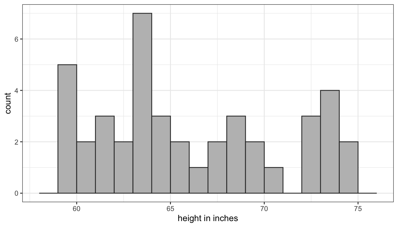
Figure 34: Population distribution of height in a class of students
The population distribution of height is bimodal which is typical, because we are mixing the heights of men and women. The population mean of height (\(\mu\)) is 66.517 inches.
Lets say I lost the results of the student survey and I wanted to know the mean height of the class. I could take a random sample of two students in order to calculate the mean height. Lets say I drew a sample of two people who were 68 and 74 inches respectively in height. I would estimate a sample mean of 71 inches which in this case would be too high. Lets say I took another sample of two students and ended up with a mean height of 66 which would be too low. Lets say I repeat this procedure until I had sampled all possible combinations of two students out of the twenty in the class.
How many samples would this be? On the first draw from the population of 42 students there are 42 possible results. On the second draw, there are 41 possible results, because I won’t re-sample the student I selected the first time. This gives me 42*41=1722 possible combinations of 42 students in two draws. However, half of these draws are just mirror images of the other draws where I swap the first and second draw. Since I don’t care about the order, I actually have 1722/2=861 possible samples.
I have used a computer routine to actually calculate the sample means in all 861 of those possible samples. The distribution of these sample means then gives us the sampling distribution of mean height for samples of size 2. Figure 35 shows a histogram of that distribution.
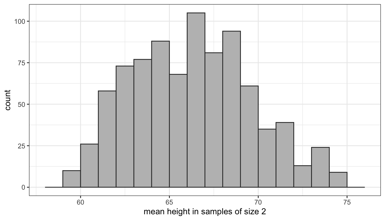
Figure 35: The sampling distribution of class height for samples of size 2
When I randomly draw one sample of size 2 and calculate its mean, I am effectively reaching into this distribution and pulling out one of these values. Note that many of the means are clustered around the true population mean of 66.5 inches, but in a few cases I can get extreme overestimates or extreme underestimates.
What if I were to increase the sample size? I have used the same computer routine to calculate the sampling distribution for samples of size 3, 4, and 5. Figure 36 shows the results.
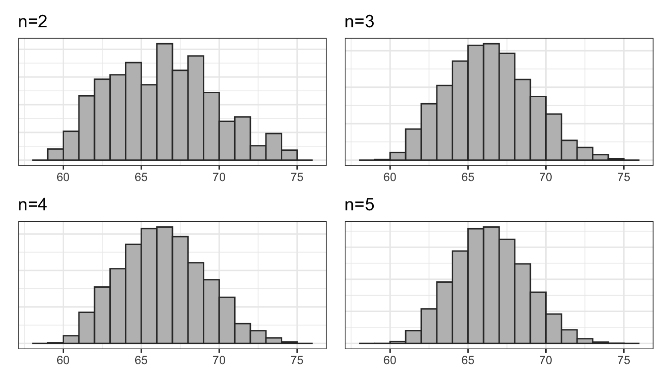
Figure 36: The sampling distribution of class height for samples of various sizes
Clearly, the shape of these distributions is changing. Another way to visualize this would be to draw density graphs which basically fit a curve to the histograms. We can then then overlap these density curves on the same graph. Figure 37 shows this graph.
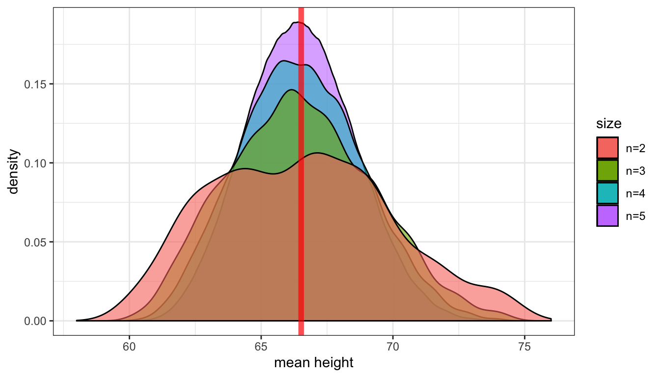
Figure 37: The sampling distribution of class height for samples of various sizes. The vertical red line shows the true population mean.
There are three thing to note here. First, each sampling distribution seems to have most of the sample means clustered (where the peak is) around the true population mean of 66.5. In fact, the mean of each of these sampling distributions is exactly the true population parameter, as I will show below. Second, the spread of the distributions is shrinking as the sample size increases. You can see that the when the sample size increases, the tails of the distribution are “pulled in” and more of the sample means are closer to the center. This indicates that we are less likely to draw a sample mean that is extremely different from the population mean in larger samples. Third, the shape of the distribution at larger sample sizes is becoming more symmetric and “bell-shaped.”
Lets take a look at the mean and standard deviation of these sampling distributions:
| Distribution | Mean | Standard Deviation |
|---|---|---|
| Population Distribution | 66.517 | 4.87 |
| Sampling Distribution (n=2) | 66.517 | 3.363 |
| Sampling Distribution (n=3) | 66.517 | 2.71 |
| Sampling Distribution (n=4) | 66.517 | 2.316 |
| Sampling Distribution (n=5) | 66.517 | 2.044 |
Note that the mean of each sampling distribution is identical to the true population mean. This is not a coincidence. The mean of the sampling distribution of sample means is always itself equal to the population mean. In statistical terminology, this is the definition of an unbiased statistic. Given that we are trying to estimate the true population mean, it is reassuring that the “average” sample mean we should get is the true population mean.
Also note that the standard deviation of the sampling distributions gets smaller with increasing sample size. This is the mathematically way of seeing the shrinking of the spread that we observed graphically. In larger sample sizes, we are less likely to draw a sample mean far away from the true population mean.
Central limit theorem and the normal distribution
The patterns we are seeing here are well known to statisticians. In fact, they are patterns that are predicted by the most important theorem in statistics, the central limit theorem. We won’t delve into the technical details of this theorem. We can generally interpret the central limit theorem to say:
As the sample size increases, the sampling distribution of a sample mean becomes a normal distribution. This normal distribution will be centered on the true population mean \(\mu\) and with a standard deviation equal to \(\sigma/\sqrt{n}\), where \(\sigma\) is the population standard deviation.
What is this “normal” distribution? The name is somewhat misleading because there is nothing particularly normal about the normal distribution. Most real-world distributions don’t look normal, but the normal distribution is central to statistical inference because of the central limit theorem. The normal distribution is a bell-shaped, unimodal, symmetric distribution. It has two characteristics that define its exact shape. The mean of the normal distribution define where its center is and the standard deviation of the normal distribution defines its spread.
Lets look at the normal sampling distribution of the mean to become familiar with it.
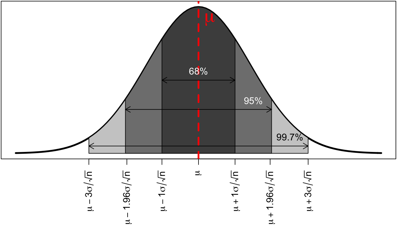
(#fig:normal_dist)The Normal Distribution
The distribution is symmetric and bell shaped. The center of the distribution is shown by the red dotted line. This center will always be at the true population mean, \(\mu\). The area of the normal distribution also has a regularity that is sometimes referred to as the “68%,95%,99.7%” rule. Regardless of the actual variable, 68% of all the sample means will be within 68% of the true population mean, 95% of all the sample means will be within 95% of the true population mean, and 99.7% of all the sample means will be within three standard deviations of the mean. This regularity will become very helpful later on for making statistical inferences.
The standard error
It is easy to get confused by the number of standard deviations being thrown around in this section. There are three standard deviations we need to keep track of to properly understand what is going on here. Each of these standard deviations is associated with one of the types of distributions I introduced at the beginning of this section.
- \(\sigma\): the population standard deviation. In our example, this would be the standard deviation of height for all 42 students which is 4.8702139. Typically, like other values in the population, this number is unknown.
- \(s\): the sample standard deviation. In our example, this would be the standard deviation of height from a particular sample of a given size from the class. This number can be calculated for the sample that you have, using the techniques we learned earlier in the class.
- \(\sigma/\sqrt{n}\): The standard deviation of the sampling distribution of the sample mean. We divide the population standard deviation \(\sigma\) by the square root of the sample size. In general, we refer to the standard deviation of the sampling distribution as the standard error, for short. So remember that when I refer to the “standard error” I am using shorthand for the “standard deviation of the sampling distribution.”
Other sample statistics
In the example here, I have focused on the sample mean as the sample statistic of interest. However, the logic of the central limit theorem applies to several other important sample statistics of interest to us. In particular, the sampling distributions of:
- means
- proportions
- mean differences
- proportion differences
- correlation coefficients
all become normal as the sample size increases. Thus, this normal distribution becomes critically important in making statistical inferences.
Note that the standard error formula \(\sigma/\sqrt{n}\) only applies to the sampling distribution of sample means. Other sample statistics have different formulas for their standard errors, which I will introduce in the next section.
What can we do with the sampling distribution?
Now that we know the sampling distribution of the sample mean should be normally distributed, what can we do with that information? The sampling distribution gives us information about how we would expect the sample means to be distributed. This seems like it should be helpful in figuring out whether we got a value close to the center or not. However, there is a catch. We don’t know either \(\mu\), the center of this distribution or \(\sigma\) which we need to calculate its standard deviation. Thus, we know theoretically what it should look like but we have no concrete numbers to determine its actual shape.
We can fix the problem with not knowing \(\sigma\) fairly easily. We don’t know \(\sigma\) but we do have an estimate of it in \(s\), the sample standard deviation. In practice, we us this value to calculate an estimated standard error of \(s/\sqrt{n}\). However, this substitution has consequences. Because we are using a sample statistic subject to random bias to estimate the standard error, this creates greater uncertainty in our estimation. I will come back to this issue in the next section.
We still have the more fundamental problem that we don’t know where the center of the sampling distribution should be. In order to make statistical inferences, we are going to employ two different methods that make use of what we do know about the sampling distribution:
- Confidence intervals: Provide a range of values within which you feel confident that the true population mean resides.
- Hypothesis tests: Play a game of make believe. If the true population mean was a given value, what is the probability that I would get the sample mean value that I actually did?
I will discuss these two different methods in the next two sections.